Design Lab 05: Get a Load Of This!
Files
This lab description is available as a PDF file here. The
code distribution may be downloaded (in zip format) here, or by
running athrun 6.01 getFiles from an Athena machine or a 6.01 lab
laptop.
1) Components
All necessary components should be available from the yellow bin at your table or from the table at the front of the room.
2) Joystick (Dual Potentiometer)
A potentiometer (or pot) is a three-terminal device whose electrical properties depend on the angle of its mechanical shaft. We can think of a potentiometer as being made up of two resistors, whose resistances sum to some value R_p, and whose resistances vary with the angle of the shaft, which we will quantify using a number \alpha: one resistor has resistance \alpha R_p, and the other has resistance (1-\alpha)R_p. Schematically, we can represent pots in the following two ways:
The quantity \alpha corresponds to the angle of the potentiometer's shaft, normalized to be in the range [0, 1]. \alpha=0 corresponds to the potentiometer's shaft being turned all the way in one direction, and \alpha increases as the shaft angle increases, until reaching \alpha=1 when the shaft is turned all the way in the other direction.
As the angle of the input shaft increases, the resistance between the bottom and middle terminals increases and the resistance between the middle and top terminal decreases. These changes in resistance occur such that the sum of the top and bottom resistors is constant.
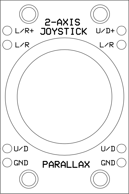
For this lab, we will use a joystick, which consists of two separate potentiometers in a single package:
This package contains two potentiometers, which are connected to the pins labeled as follows:
Notice that the joystick has two degrees of freedom. Moving the joystick along one of its axes changes \alpha_1, and moving the joystick along the other axis changes \alpha_2.
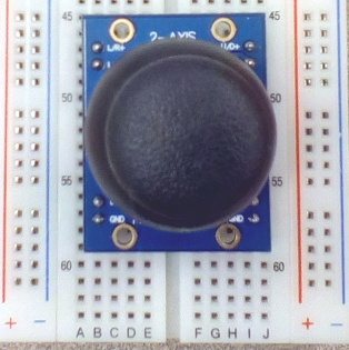
Plug the joystick in to your breadboard as shown in the picture below:

Note that there should be one row of holes on either side of the joystick package.
To begin, we will start by considering only the pot between U/D+ and GND.
Use your multimeter to measure the
total internal resistance R_p of the potentiometer between U/D+ and GND
on the joystick.
U/D+ and GND on
the joystick, and enter the result below, in Ohms:
R_p =~
3) Divide and Conquer
Our ultimate goal for this lab is to drive the robot around using the joystick. To do this, we would like to be able to set the robot's forward and rotational velocities based on the \alpha values of each of the potentiometers in the joystick. To accomplish this, we would like to be able to measure these \alpha values directly; but unfortunately, we can't. What we can do, however, is to create a voltage that varies as \alpha varies, and to use this voltage to figure out the \alpha values.
Consider connecting this single potentiometer as a voltage divider, as illustrated below (showing both models of the potentiometer):
3.1) Solving
For the voltage divider configuration above, what is the value of V_o we expect (in Volts) when \alpha=0? When \alpha=1? When \alpha=0.5? Note that there is extra scratch paper attached to the end of the handout.Enter your answers as decimal numbers accurate to within 10^{-3} Volts. Note that these boxes will accept Python expressions as well as individual numbers, so you do not need to simplify your answer completely. Since Python is doing the interpretation, be careful of integer division!
4) Interfacing
In this section, we will get some practice with using a circuit to interface with the robot.
4.1) Connect to the Robot
We can power our circuit from the robot by using an 8-pin Connector; one should be available from a yellow bin at your table. The robot provides a 10-volt power supply, which you can access through pins 2 (+10V) and 4 (0V) of the robot connector.
Construct a variable voltage divider (as shown above, connecting to the pins
labeled U/D+ and GND) on a protoboard, using the robot to provide +10V
and ground. Note that it may be easiest first to connect pins 2 and 4 of the
robot connector to the red and blue rails on the protoboard, and then to use
those rails to provide power and ground to the rest of your circuit.
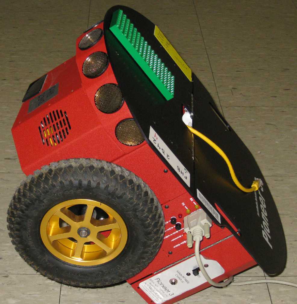
Connect the long CAT-5 cable (the same kind of cable that is used for Ethernet) from the top of the robot into the 8-pin connector, and power the robot on (this will provide power to your circuit).
U/D). What is this voltage when the joystick is in its
neutral location? How does it change as you move the joystick?
The robot also contains an analog-to-digital
converter (ADC), which can be used to measure voltages. The voltages on 1,
3, 5, and 7 of the robot connector are stored in a tuple called robot.analogs.
A complete pinout for the robot connector is provided on the last page of
the PDF handout.
Add a connection to your circuit so that the voltage V_o is being measured by analog input 1 on the robot (pin 1 of the connector).
4.2) Sweep
Run the soar brain potInputBrain.py (located in this week's distribution).
This brain will have the robot stand still and collect measurements from analog input
1, for up to 20 seconds. After the brain is stopped (by clicking the stop button),
soar will generate a plot of how the input varied with time.
Move the pot to \alpha = 0, click "start", and generate a "sweep" by moving the pot smoothly from \alpha = 0 to \alpha = 1 as the brain is running. Save the plot generated by soar!
If you need to run the sweep multiple times, make sure to click the "Reload Brain And World" button in between trials.
4.3) Gotta Go Fast

Now, we will program the robot to set its forward velocity based on the
position of the potentiometer. Modify the on_step function in
potInputBrain.py so that the robot moves forward with a velocity
proportional to \alpha - \alpha_{center}, where
\alpha_{center} is the value of \alpha when the joystick
is centered. When \alpha=1, the robot should drive
quickly forward; when \alpha=0.5, the robot should stand still;
and when \alpha=0, the robot should drive quickly backward. A
good constant of proportionality to start with is 0.5.
Once you are reasonably sure your robot will move as expected, set its wheels back down, and try using the pot to move it around. Does it move as you would expect?
5) To Everything There Is A Season
Our next goal is to develop a means of steering the robot using circuit-based controls. The joystick on your breadboard has a second potentiometer (for the orthogonal axis of movement) that can be used for steering, using an approach similar to what we did for forward velocity.
To let the robot act upon this steering signal, use one of the remaining Analog
Inputs on the robots (see Pin Diagram in reference image) to measure the
voltage. Note also that the two pins labeled GND are already connected
together, so you do not need to separately connect each to our the 0V from
the robot connector.
6) Loading...
Now, let's add an indicator light to our breadboard. This light should be on at its maximum when the robot is moving forward at top speed, completely off when the robot is moving backward at top speed. We can do this by connecting a light bulb up to the voltage on pin 1 (call it V_{i_1}), so that the light is brightest when there is a large voltage at that point, and off when the voltage at that point is 0V.
Do this by wiring up a 470\Omega resistor and a green LED (light-emitting diode) as shown in the following diagram, where V_{i_1} is the voltage at the center of the potentiometer (or the voltage at pin 1 of the robot connector). Importantly, the longer lead of the LED should be connected to the resistor, not to ground. Do not cut the leads of the LED.
Try driving the robot now that the indicator light is in place. What is different about the robot's behavior now?
Note that you do not have to fix this behavior right now (we'll work on that later on in the lab), but you should be prepared to discuss these differences during a checkoff.
6.1) Sweep
Prevent the robot from moving and generate another graph of how V_{i_1} changes as \alpha changes, as you did earlier. Save this plot.
Demonstrate your driving robot to a staff member, with and without the indicator light. What changed when you included the indicator light? Can you explain this difference?
7) Correction
In the previous checkoff, we noticed that, with the addition of the light, the way in which V_{i_1} depends on \alpha changed, and so our initial means of converting between the two will no longer work. Since we would still like the robot's speed to be proportional to \alpha, we will need to determine the relationship between them in order for our control scheme to work.
In order to understand this relationship, we will need a way to model the circuit we have built. This is complicated by the fact that an LED is a nonlinear device. However, as we often did in the LTI labs, we can approximate the LED in the context of this circuit using linear devices. Here are some data collected by measuring the voltage drop across the LED as we vary \alpha in this circuit:
(For a voltage source, enter your answer in Volts; for a resistor, enter your answer in Ohms)
Note that you may need to make a measurement to determine this value.
In the handout, draw a schematic diagram of the circuit for driving the robot forward and back (including the potentiometer and the indicator light), using your linear model of the diode. You may wish to check your diagram with a staff member before moving on.
7.1) Compensation
Our goal is to programmatically estimate \alpha (which represents the position of the potentiometer) from a measured voltage V_{i_1} so that we can base our proportional controller off of the position of the pot (remember that we want a linear relationship between \alpha and the robot's forward velocity, but after adding the indicator, our controller does not have that property).
In this circuit, though, determining $\alpha$ from a given $V_{i_1}$ analytically is, in fact, quite complicated. Luckily, finding $V_{i_1}$ given $\alpha$ is much easier. As such, we will first write a function to determine $V_{i_1}$ for a given $\alpha$ value, and then we will use that to back-solve for the value of $\alpha$ associated with a particular voltage.In potInputBrain.py, complete the definition of the function
voltage_from_alpha(alpha, v_d, r_p). This function should take three
inputs: a value of \alpha; a voltage representing the constant
voltage of the voltage source we are using to model the diode, in Volts; and a
resistance representing the total resistance of the potentiometer, in Ohms. Your
function should return the voltage at the output of the potentiometer, in
Volts.
You may find it helpful to give each resistance a name (e.g., R_1, R_2, and R_3), and to solve in terms of those variables, rather than solving the entire circuit in terms of R_p, \alpha, etc.
voltage_from_alpha below.
Remember that our goal was to estimate \alpha, given a measured voltage.
We are trying to find the value of alpha that makes
voltage_from_alpha(alpha, ...) be as close as possible to the measured
voltage.
\alpha = 0, 0.01, 0.02, \ldots, 0.99, 1. Does the graph look like you would expect? Note that there is some example code for generating plots, commented out near the bottom of the brain file.
voltage_from_alpha to do this?
If you are having trouble, please ask a staff member for help.
In potInputBrain.py, complete the definition of the function
alpha_from_voltage(voltage, v_d, r_p), which should take in a voltage as
measured by the robot, and return the value of \alpha that we expect would
have generated that voltage.
alpha_from_voltage below.
alpha_from_voltage on voltages range from 0V to 10V. How would you expect this graph to compare to your graph of voltage vs \alpha?
7.2) Driving
Finally, update the driving code in your soar brain to make use of your
alpha_from_voltage function. Your brain should measure the voltage on
the analog input, and use that to determine an estimated value of
\alpha. It should then use this value of \alpha to
determine how fast the robot should move.
Test your driving code on the real robot. How does its behavior compare, before and after your corrections?
Can you get your robot to follow one of the lines
on the floor accurately? Can you get it to trace "MIT?" Note that soar will
generate a second plot showing the robot's path through the world if you set
bread_crumbs = True in the soar brain.
Discuss the results of your compensation experiments with a staff member. Demonstrate your working robot.
8) Optional: Light Refreshment
If you have time, add turn signals to your robot, because that will help the robot be a productive member of society and not disrespect other robots, which is what not using your turn signals says about a person. Grab two orange LEDs from the bin up front. In addition, grab two 470\Omega resistors. Build the circuit shown below, using the orthogonal potentiometer on your joystick. Once this is completed, test your circuit by ensuring that the two LEDs light up in alternating ways when you turn your pot in the turn direction.
8.1) Sweep
Prevent the robot from moving and generate another graph of how this voltage changes as \alpha changes, as you did earlier. Note that you may need to change your code slightly to measure the right voltage.
Discard all resistors and bent wires.
Put pots, connectors, LEDs, and unbent wires back in appropriate places.