6.01 Course Notes

Imagine that you are asked to design a system to steer a car straight down the middle of a lane. It seems easy, right? You can figure out some way to sense the position of the car within its lane. Then, if the car is right of center, turn the steering wheel to the left. As the car moves so that it is less to the right, turn the steering wheel less to the left. If it is left of center, turn the steering wheel to the right. This sort of proportional controller works well for many applications, but not for steering, as can be seen below.

It is relatively easy to describe better algorithms in terms that humans would understand: e.g., Stop turning back and forth! It is not so easy to specify exactly what one might mean by that, in a way that it could be automated. In this chapter, we will develop a Signals and Systems framework to facilitate reasoning about the dynamic behaviors of systems. This framework will enable construction of simple mathematical models that are useful in both analysis and design of a wide range of systems, including the car-steering system.

1.2) The Signals and Systems Abstraction

To think about dynamic behaviors of systems, we need to think not only about how to describe the system but also about how to describe the signals that characterize the inputs and outputs of the system, as illustrated below.

This diagram represents a system with one input and one output. Both the input and output are signals. A signal is a mathematical function with an independent variable (most often it will be time for the problems that we will study) and a dependent variable (that depends on the independent variable). The system is described by the way that it transforms the input signal into the output signal. In the simplest case, we might imagine that the input signal is the time sequence of steering-wheel angles (assuming constant speed) and that the output signal is the time sequence of distances between the center of the car and the midline of the lane.

Representing a system with a single input signal and a single output signal seems too simplistic for any real application. For example, the car in the steering example (in the figure above) surely has more than one possible output signal.

Check Yourself 1:

List at least four possible output signals for the car-steering problem.

Show/Hide

Possible output signals include

its three-dimensional position (which could be represented by a 3D vector $\hat{p}(t)$ or by three scalar functions of time),
its angular position,
the rotational speeds of the wheels,
the temperature of the tires, and many other possibilities.

The important point is that the first step in using the signals and systems representation is abstraction: we must choose the output(s) that are most relevant to the problem at hand and abstract away the rest. To understand the steering of a car, one vital output signal is the lateral position p_ o(t) within the lane, where p_ o(t) represents the distance (in meters) from the center of the lane. That signal alone tells us a great deal about how well we are steering. Consider a plot of p_ o(t) that corresponds to the figure above, as follows.

The oscillations in p_ o(t) as a function of time correspond to the oscillations of the car within its lane. Thus, this signal clearly represents an important failure mode of our car steering system. Is p_ o(t) the only important output signal from the car-steering system? The answer to this question depends on your goals. Analyzing a system with this single output is likely to give important insights into some systems (e.g., low-speed robotic steering) but not others (e.g., NASCAR). More complicated applications may require more complicated models. But all useful models focus on the most relevant signals and ignore those of lesser significance ¹. Throughout this chapter, we will focus on systems with one input signal and one output signal. When multiple output signals are important for understanding a problem, we will find that it is possible to generalize the methods and results developed here for single-input and single-output systems to systems with multiple inputs and outputs. The signals and systems approach has very broad applicability: it can be applied to mechanical systems (such as mass-spring systems), electrical systems (such as circuits and radio transmissions), financial systems (such as markets), and biological systems (such as insulin regulation or population dynamics). The fundamental notion of signals applies no matter what physical substrate supports them: it could be sound or electromagnetic waves or light or water or currency value or blood sugar levels.

1.2.1) Modularity, primitives, and composition

The car-steering system can be analyzed by thinking of it as the combination of car and steering sub-systems. The input to the car is the angle of the steering wheel. Let's call that angle \phi (t) . The output of the car is its position in the lane, p_ o(t), measured as the lateral distance to the center of the lane.

The steering controller turns the steering wheel to compensate for differences between our desired position in the lane, p_ i(t) (which is zero since we would like to be in the center of the lane), and our actual position in the lane p_ o(t). Let e(t)=p_ i(t)-p_ o(t). Thus, we can think about the steering controller as having an input e(t) and output \phi (t).

In the composite system (below), the steering controller determines \phi (t), which is the input to the car. The car generates p_ o(t), which is subtracted from p_ i(t) to get e(t), which is the input to the steering controller. The triangular component is called a gain or scale of -1: its output is equal to -1 times its input. More generally, we will use a triangle symbol to indicate that we are multiplying all the values of the signal by a numerical constant, which is shown inside the triangle.

The dashed-red box in the figure above illustrates modularity of the signals and systems abstraction. Three single-input, single-output sub-systems (steering controller, car, and inverter) and an adder (two inputs and 1 output) are combined to generate a new single-input (p_ i(t)), single-output (p_ o(t)) system. By abstraction, we could treat this new system as a primitive (represented by a single-input single-output box) and combine it with other subsystems to create a new, more complex, system. A principal goal of this chapter is to develop methods of analysis for the sub-systems that can be combined to analyze the overall system.

1.2.2) Discrete-time signals and systems

This chapter focuses on signals whose independent variables are discrete (e.g., take on only integer values). Some such signals are found in nature. For example, the primary structure of DNA is described by a sequence of base-pairs. However, we are primarily interested in discrete-time signals, not so much because they are found in nature, but because they are found in computers. Even though we focus on interactions with the real world, these interactions will primarily occur at discrete instants of time. For example, the difference between our desired position p_ i(t) and our actual position p_ o(t) is an error signal e(t), which is a function of continuous time t. If the controller only observes this signal at regular sampling intervals T, then its input could be regarded as a sequence of values x[n] that is indexed by the integer n. The relation between the discrete-time sequence x[n] (note square brackets) and the continuous signal x(t) (note round brackets) is given by x[n] = x(nT), where T is the length of one timestep, which we call the sampling relation. Sampling converts a signal of continuous domain to one of discrete domain. While our primary focus will be on time signals, sampling works equally well in other domains. For example, images are typically represented as arrays of pixels accessed by integer-valued rows and columns, rather than as continuous brightness fields, indexed by real-valued spatial coordinates. If the car-steering problem in the beginning were modeled in discrete time, we could describe the system with a diagram that is very similar to the continuous-time diagram above. However, only discrete time instants are considered and the output position is now only defined at discrete times, as shown below.

1.2.3) Linear, Time-Invariant Systems

We will be focusing our attention on a specific class of systems: discrete-time linear time-invariant (LTI) systems. In the first few labs, we will see how it is possible to simulate these kinds of systems; what's more, we will see that limiting our attention to this subclass of systems will allow us to predict the behavior of such systems without even simulating them, which will allow deeper forms of analysis. In an LTI system:

The output at time n is a linear combination of previous and current inputs, and previous outputs.
The behavior of the system does not depend on the absolute time at which it was started.

We are particularly interested in LTI systems because they can be analyzed mathematically, in a way that lets us characterize some properties of their output signal for any possible input signal. This is a much more powerful kind of insight than can be gained by trying a machine out with several different inputs. Another important property of LTI systems is that they are compositional: the cascade, parallel, and feedback combinations of LTI system are themselves LTI systems.

1.3) Discrete-time Signals

In this section, we will work through the PCAP system for discrete time signals, by introducing a primitive and three methods of composition, and the ability to abstract by treating composite signals as if they themselves were primitive. A signal is an infinite sequence of sample values at discrete time steps. We will use the following common notational conventions: A capital letter X stands for the whole input signal and x[n] stands for the value of signal X at time step n

It is conventional, if there is a single system under discussion, to use X for the input signal to that system and Y for the output signal.

We will say that systems transduce input signals into output signals.

1.3.1) Unit sample signal

We will work with a single primitive, called the unit sample signal, \Delta . It is defined on all positive and negative integer indices as follows ²:

\delta[n] = \begin{cases} 1 & \text{if}~n=0 \\ 0 & \text{otherwise} \end{cases}

That is, it has value 1 at index n=0 and 0 otherwise, as shown below:

1.3.2) Signal Combinators

1.3.2.1) Scaling

Our first operation will be scaling, or multiplication by a scalar. A scalar is any real number. The result of multiplying any signal X by a scalar c is a signal, so that,

if Y = c \cdot X, then y[n] = c \cdot x[n]

That is, the resulting signal has a value at every index n that is c times the value of the original signal at that location. Here are the signals 4 \Delta and -3.3 \Delta:

1.3.2.2) Delay

The next operation is the delay operation. The result of delaying a signal X is a new signal \mathcal{R} X such that:

if Y = \mathcal{R} X then y[n] = x[n-1].

That is, the resulting signal has the same values as the original signal, but delayed by one step in time. You can also think of this, graphically, as shifting the signal one step to the Right. Here is the unit sample delayed by 1 and by 3 steps. We can describe the second signal as \mathcal{R} \mathcal{R} \mathcal{R} \Delta, or, using shorthand, as \mathcal{R} ^3\Delta.

1.3.2.3) Addition

Finally, we can add two signals together. Addition of signals is accomplished component-wise, so that:

if Y = X_1 + X_2 then y[n] = x_1[n] + x_2[n]

That is, the value of the composite signal at step n is the sum of the values of the component signals. Here are some new signals constructed by summing, scaling, and delaying the unit sample.

Note that, because each of our operations returns a signal, we can use their results again as elements in new combinations, showing that our system has true compositionality. In addition, we can abstract, by naming signals. So, for example, we might define Y = 3\Delta + 4\mathcal{R} \Delta - 2\mathcal{R} ^2\Delta, and then make a new signal Z = Y + 0.3\mathcal{R} Y, which would look like this:

Be sure you understand how the heights of the spikes are determined by the definition of Z .

Check Yourself 2:

Draw a picture of samples -1 through 4 of Y - \mathcal{R} Y.

It is important to remember that, because signals are infinite objects, these combination operations are abstract mathematical operations. You could never somehow 'make' a new signal by calculating its value at every index. It is possible, however, to calculate the value at any particular index, as it is required.

1.3.3) Algebraic Properties of Operations on Signals

Adding and scaling satisfy the familiar algebraic properties of addition and multiplication: addition is commutative and associative, scaling is commutative (in the sense that it doesn't matter whether we pre- or post-multiply) and scaling distributes over addition:

c\cdot (X_1+X_2)=c\cdot X_1 + c \cdot X_2

which can be verified by defining Y = c\cdot (X_1+X_2) and Z = c\cdot X_1 + c \cdot X_2 and checking that y[n] = z[n] for all n:

y[n] = z[n]

c\cdot (x_1[n] + x_2[n]) = (c\cdot x_1[n]) + (c\cdot x_2[n])

which clearly holds based on algebraic properties of arithmetic on real numbers. In addition, \mathcal{R} distributes over addition and scaling, so that:

\mathcal{R}(X_1 + X_2) = \mathcal{R}X_1 + \mathcal{R}X_2

\mathcal{R}(c\cdot X) = c\cdot (\mathcal{R}X)

Check Yourself 3:

Verify that \mathcal{R} distributes over addition and multiplication by checking that the appropriate relations hold at some arbitrary step n.

These algebraic relationships mean that we can take any finite expression involving \Delta, \mathcal{R} + and \cdot and convert it into the form

(a_ o + a_1\mathcal{R} ^1 + a_2\mathcal{R} ^2 + \ldots + a_ N \mathcal{R} ^{N}) \Delta

That is, we can express the entire signal as a polynomial in \mathcal{R}, applied to the unit sample. In our previous example, it means that we can rewrite 3\Delta + 4\mathcal{R} \Delta - 2\mathcal{R} ^2\Delta as (3 + 4\mathcal{R} - 2\mathcal{R} ^2)\Delta.

1.4) Feedforward systems

We will start by looking at a subclass of discrete-time LTI system, which are exactly those that can be described as performing some combination of scaling, delay, and addition operations on the input signal. We will develop several ways of representing such systems, and see how to combine them to get more complex systems in this same class.

1.4.1) Representing systems

We can represent systems using operator equations, difference equations, block diagrams, and Python state machines. Each makes some things clearer and some operations easier. It is important to understand how to convert between the different representations.

1.4.1.1) Operator equation

An operator equation is a description of how signals are related to one another, using the operations of scaling, delay, and addition on whole signals. Consider a system that has an input signal X, and whose output signal is X - \mathcal{R} X. We can describe that system using the operator equation

Y = X - \mathcal{R} X

Using the algebraic properties of operators on signals described in the section on "Algebraic properties of operations on signals", we can rewrite this as

Y = (1 - \mathcal{R}) X

which clearly expresses a relationship between input signal X and output signal Y, whatever X may be.

Feedforward systems can always be described using an operator equation of the form Y = \Phi X, where \Phi is a polynomial in \mathcal{R}.

1.4.1.2) Difference Equation

An alternative representation of the relationship between signals is a difference equation. A difference equation describes a relationship that holds among samples (values at particular times) of signals. We use an index n in the difference equation to refer to a particular time index, but the specification of the corresponding system is that the difference equation hold for all values of n

The operator equation
Y = X - \mathcal{R} X
can be expressed as this equivalent difference equation:
y[n] = x[n] - x[n-1]
The operation of delaying a signal can be seen here as referring to a sample of that signal at time step n-1
Difference equations are convenient for step-by-step analysis, letting us compute the value of an output signal at any time step, given the values of the input signal.

So, if the input signal X is the unit sample signal,

x[n] = \delta[n] = \begin{cases} 1 & ~\text{if}~n=0 \\ 0 & ~\text{otherwise} \end{cases}

then, using a difference equation, we can compute individual values of the output signal Y:

y[n] = x[n] - x[n-1]

\begin{align} y[0] & = x[0] - x[-1] & = 1 - 0 & = 1 \\ y[1] & = x[1] - x[0] & = 0 - 1 & = -1 \\ y[2] & = x[2] - x[1] & = 0 - 0 & = 0 \\ y[3] & = x[3] - x[2] & = 0 - 0 & = 0 \\ \end{align}

1.4.1.3) Block Diagrams

Another way of describing a system is by drawing a block diagram, which is made up of components,connected by lines with arrows on them. The lines represent signals; all lines that are connected to one another (not going through a round, triangular, or circular component) represent the same signal.The components represent systems. There are three primitive components corresponding to our operations on signals:

Delay components are drawn as rectangles, labeled Delay, with two lines connected to them, one with an arrow coming in and one going out. If X is the signal on the line coming into the delay, then the signal coming out is RX.
Scale(or gain) components are drawn as triangles, labeled with a positive or negative number c, with two lines connected to them, one with an arrow coming in and one going out. If X is the signal on the line coming into the gain component, then the signal coming out is c \cdot X
Adder components are drawn as circles, labeled with+, three lines connected to them, two with arrows coming in and one going out. If X_1 and X_2 are the signals on the lines point into the adder, then the signal coming out is X_1+X_2.

For example, the system Y = X-{\cal R}X can be represented with this block diagram:

1.4.2) Combinations of systems

To combine LTI systems, we will use the same cascade and parallel-add operations as we had for state machines.

1.4.2.1) Cascade multiplication

When we make a cascade combination of two systems, we let the output of one system be the input of another. So, if the system M_1 has operator equation Y = \Phi _1X and system M_2 has operator equation Z = \Phi _2 W , and then we compose M_1 and M_2 in cascade by setting Y = W , then we have a new system, with input signal X , output signal Z , and operator equation Z = (\Phi _2 \cdot \Phi _1) X

The product of polynomials is another polynomial, so \Phi _2 \cdot \Phi _1 is a polynomial in \mathcal{R}
Furthermore, because polynomial multiplication is commutative, cascade combination is commutative as well (as long as the systems are at rest, which means that their initial states are 0).

So, for example,

\mathcal{R}(1-\mathcal{R})\, X=(1-\mathcal{R})\mathcal{R} X

and these two corresponding block diagrams are equivalent (the algebraic equivalence justifies the diagram equivalence):

Cascade combination, because it results in multiplication, is also associative, which means that any grouping of cascade operations on systems has the same result.

1.4.2.2) Parallel addition

When we make a parallel addition combination of two systems, the output signal is the sum of the output signals that would have resulted from the individual systems. So, if the system M_1 is represented by the equation Y = \Phi _1X and system M_2 is represented by the equation Z = \Phi _2 X, and then we compose M_1 and M_2 with parallel addition by setting output W = Y + Z, then we have a new system, with input signal X, output signal W, and operator equation W = (\Phi _1 + \Phi _2) X. Because addition of polynomials is associative and commutative, then so is parallel addition of feed-forward linear systems.

1.4.2.3) Combining cascade and parallel operations

Finally, the distributive law applies for cascade and parallel combination, for systems at rest, in the same way that it applies for multiplication and addition of polynomials, so that if we have three systems, with operator equations:

\begin{align} Y & = \Phi_1 X \\ U & = \Phi_2 Y \\ W & = \Phi_3 Z \\ \end{align}

and we form a cascade combination of the sum of the first two, with the third, then we have a system describable as:

B = (\Phi _3 \cdot (\Phi _1 + \Phi _2)) A

We can rewrite this, using the distributive law, as:

B = ((\Phi _3 \cdot \Phi _1) + (\Phi _3 \cdot \Phi _2)) A

So, for example,

\mathcal{R}(1-\mathcal{R})=\mathcal{R}-\mathcal{R}^2

and these two corresponding block diagrams are equivalent:

Here is another example of two equivalent operator equations

(\mathcal{R} - \mathcal{R}^2)(2 - \mathcal{R}) X = (1 - \mathcal{R})(2\mathcal{R} - \mathcal{R}^2) X

and these two corresponding block diagrams are equivalent if the systems start at rest:

Check Yourself 4:

Convince yourself that all of these systems are equivalent. One strategy is to convert them all to operator equation representation.

1.5) Feedback Systems

So far, all of our example systems have been _feedforward_: the dependencies have all flowed from the input through to the output, with no dependence of an output on previous output values. In this section, we will extend our representations and analysis to handle the general class of LTI systems in which the output can depend on any finite number of previous input or output values.

1.5.1) Accumulator example

Consider this block diagram, of an accumulator:

It's reasonably straightforward to look at this block diagram and see that the associated difference equation is

y[n] = x[n] + y[n-1]

because the output on any given step is the sum of the the input on that step and the output from the previous step. Let's use the difference equation to understand what the output of this system is when the input is the unit sample signal. To compute the output at step n, we need to evaluate

y[n] = x[n] + y[n-1]

We immediately run up against a question: what is the value of y[n-1]? The answer clearly has a profound effect on the output of the system. In our treatment of feedback systems, we will generally assume that they start 'at rest', which means that all values of the inputs and outputs at steps less than 0 are 0. That assumption lets us fill in the following table:

\begin{align} y[n] & = x[n] + y[n-1] & & \\ y[0] & = x[0] + y[-1] & = 1 + 0 & = 1\\ y[1] & = x[1] + y[0] & = 0 + 1 & = 1\\ y[2] & = x[2] + y[1] & = 0 + 1 & = 1\\ \end{align}

Here are plots of the input signal X and the output signal Y:

This result may be somewhat surprising! In feedforward systems, we saw that the output was always a finite sum of scaled and delayed versions of the input signal; so that if the input signal was transient (had a finite number of non-zero samples) then the output signal would be transient as well. But, in this feedback system, we have a transient input with a persistent (infinitely many non-zero samples) output. We can also look at the operator equation for this system. Again, reading it off of the block diagram, it seems like it should be

Y = X + \mathcal{R} Y

It's a well-formed equation, but it isn't immediately clear how to use it to determine Y. Using what we already know about operator algebra, we can rewrite it as:

Y(1 - \mathcal{R}) = X

which defines Y to be the signal such that the difference between Y and \mathcal{R} Y is X. But how can we find that Y?

We will now show that we can think of the accumulator system as being equivalent to another system, in which the output is the sum of infinitely many feedforward paths, each of which delays the input by a different, fixed value. This system has an operator equation of the form

Y=(1+\mathcal{R}+\mathcal{R}^2+\mathcal{R}^3+\cdots )X

and can be represented with a block diagram of the form:

These systems are equivalent in the sense that if each is initially at rest, they will produce identical outputs from the same input. We can see this by taking the original definition and repeatedly substituting in the definition of Y in for its occurrence on the right hand side:

\begin{align} Y & = X + {\cal R} Y \\ & = X + \mathcal{R} (X + \mathcal{R} Y) \\ & = X + \mathcal{R} (X + \mathcal{R} (X + \mathcal{R} Y))\\ & = X + \mathcal{R} (X + \mathcal{R} (X + \mathcal{R} (X + \mathcal{R} Y))) \\ Y & = (1 +\mathcal{R} + \mathcal{R}^2 + \mathcal{R}^3 + \ldots ) X \\ \end{align}

Now, we can informally derive a 'definition' of the reciprocal of 1 - \mathcal{R} (the mathematical details underlying this are subtle and not presented here),

\frac{1}{1-\mathcal{R}} = 1+\mathcal{R}+\mathcal{R}^2+\mathcal{R}^3+\cdots

In the following it will help to remind ourselves of the derivation of the formula for the sum of an infinite geometric series:

\begin{align} S & = 1 + x + x^2 + x^3 + \cdots \\ Sx & = x + x^2 + x^3 + x^4 + \cdots \\ \end{align}

Subtracting the second equation from the first we get

S(1-x) = 1

And so, provided |x| \lt 1,

\frac{1}{1-x} = 1 + x + x^2 + x^3 + \cdots

Similarly, we can consider the system O, where

\begin{align} O & = 1 + \mathcal{R}+\mathcal{R}^2+\mathcal{R}^3+\cdots \\ {\cal R}O & = \mathcal{R}+\mathcal{R}^2+\mathcal{R}^3+\cdots\\ \end{align}

(1-\mathcal{R})O = 1

And so,

\frac{1}{1-{\cal R}} = 1 + \mathcal{R} + \mathcal{R}^2 + \mathcal{R}^3 + \cdots

Check Yourself 5:

Check this derivation by showing that

(1 + \mathcal{R} + \mathcal{R}^2 + \mathcal{R}^3 + \cdots )(1 - \mathcal{R}) = 1

So, we can rewrite the operator equation for the accumulator as

Y = \frac{1}{1-\mathcal{R}}X

We don't have an intuitive way to interpret this relationship between X and Y yet, but we will spend most of the rest of this chapter on developing intuition and analysis for systems with feedback.

1.5.2) General form of LTI systems

We can now treat the general case of LTI systems, including feedback. In general, LTI systems can be described by difference equations of the form:

y[n] = c_0y[n-1] + c_1y[n-2] + \ldots + c_{k-1}y[n-k] + d_0x[n] + d_1x[n-1] + \ldots + d_ jx[n-j]

The state of this system consists of the k previous output values and j previous input values. The output y[n] is a linear combination of the k previous output values, y[n-1], \ldots , y[n-k], j previous input values, x[n-1], \ldots , x[n-j], and the current input, x[n].

1.5.3) System Functionals

Now, we are going to engage in a shift of perspective. We started by defining a new signal Y in terms of an old signal X, much as we might, in algebra, define y = x + 6. Sometimes, however, we want to speak of the relationship between x and y in the general case, without a specific x or y in mind. We do this by defining a function f: f(x) = x + 6

We can do the same thing with LTI systems, by defining system functionals. If we take the general form of an LTI system given in the previous section and write it as an operator equation, we have

\begin{align} Y & = c_0 \mathcal{R} Y + c_1 \mathcal{R}^2 Y + \ldots + c_{k-1} \mathcal{R}^ k Y + d_0 X + d_1 \mathcal{R} X + \ldots + d_ j \mathcal{R}^ j X \\ & = (c_0 \mathcal{R} + c_1 \mathcal{R}^2 + \ldots + c_{k-1} \mathcal{R}^ k) Y+ (d_0 + d_1 \mathcal{R} + \ldots + d_ j \mathcal{R}^ j) X \\ \end{align}

We can rewrite this as

(1 - c_0 \mathcal{R} - c_1 \mathcal{R}^2 - \ldots - c_{k-1} \mathcal{R}^ k) Y = (d_0 + d_1 \mathcal{R} + \ldots + d_ j \mathcal{R}^ j) X

{Y\over X}={d_0+d_1\mathcal{R}+d_2\mathcal{R}^2+d_3\mathcal{R}^3+\cdots \over 1 - c_0\mathcal{R} - c_1\mathcal{R}^2 - c_2\mathcal{R}^3 - \cdots }

which has the form

{Y\over X} = {N(\mathcal{R})\over D(\mathcal{R})}

where N(\mathcal{R}), the numerator, is a polynomial in \mathcal{R}, and D(\mathcal{R}), the denominator, is also a polynomial in \mathcal{R}. We will refer to Y / X as the system functional: it characterizes the operation of a system, independent of the particular input and output signals involved. It is functional in the sense that it is itself an operator which can be applied to arbitrary input signals.

The system functional is most typically written in the form

{Y\over X}={b_0+b_1\mathcal{R}+b_2\mathcal{R}^2+b_3\mathcal{R}^3+\cdots \over a_0+a_1\mathcal{R}+a_2\mathcal{R}^2+a_3\mathcal{R}^3+\cdots }

where c_ i = - a_{i+1} / a_0 and d_ i = b_ i / a_0. It can be completely characterized by the coefficients of the denominator polynomial, a_ i, and the coefficients of the numerator polynomial, b_ i. It is always possible to rewrite this in a form in which a_0 = 1. Feedforward systems have no dependence on previous values of Y, so they have D(\mathcal{R}) = 1. Feedback systems have persistent behavior, which is determined by D(\mathcal{R}).

1.5.4) Primitive Systems

Just as we had a PCAP system for signals, we have one for LTI system, in terms of system functionals, as well. We can specify system functionals for each of our system primitives. A gain element is governed by operator equation Y = kX, for constant k, so its system functional is

{\cal H} = \frac{Y}{X} = k

A delay element is governed by operator equation Y = \mathcal{R} X, so its system functional is

{\cal H} = \frac{Y}{X} = \mathcal{R}

1.5.5) Combining System Functionals

We have three basic composition operations: sum, cascade, and feedback. This PCAP system, as our previous ones have been, is _ compositional_, in the sense that whenever we make a new system functional out of existing ones, it is a system functional in its own right, which can be an element in further compositions.

1.5.5.1) Addition

The system functional of the sum of two systems is the sum of their system functionals. So, given two systems with system functionals {\cal H}_1

and {\cal H}_2, connected like this:

and letting

Y_1 = {\cal H}_1 X~\text{and}~Y_2 = {\cal H}_2 X

we have

\begin{align} Y & = Y_1 + Y_2 \\ & = {\cal H}_1 X + {\cal H}_2 X\\ & = ({\cal H}_1 + {\cal H}_2) X\\ & = {\cal H} X\\ \end{align}

where {\cal H} = {\cal H}_1 + {\cal H}_2.

1.5.5.2) Cascade

The system functional of the cascade of two systems is the product of their system functionals. So, given two systems with system functionals {\cal H}_1 and {\cal H}_2, connected like this:

and letting

W = {\cal H}_1 X ~\text{and}~Y = {\cal H}_2 W

we have

\begin{align} Y & = {\cal H}_2 W\\ & = {\cal H}_2 {\cal H}_1 X \\ & = {\cal H} X \\ \end{align}

where {\cal H} = {\cal H}_2 {\cal H}_1. And note that, as was the case with purely feedforward systems, cascade combination is still commutative, so it doesn't matter whether {\cal H}_1 or {\cal H}_2 comes first in the cascade. This surprising fact holds because we are only considering LTI systems starting at rest; for more general classes of systems, such as the general class of state machines we have worked with before, the ordering of a cascade does matter.

1.5.5.3) Feedback

There are several ways of connecting systems in feedback. Here we study a particular case of negative feedback combination, which results in a classical formula called Black's formula. Consider two systems connected like this

and pay careful attention to the negative sign on the feedback input to the addition. It is really just shorthand; the negative sign could be replaced with a gain component with value -1. This negative feedback arrangement is frequently used to model a case in which X is a desired value for some signal and Y is its actual value; thus the input to {\cal H}_1 is the difference between the desired an actual values, often called an error signal. We can simply write down the operator equation governing this system and use standard algebraic operations to determine the system functional:

\begin{align} Y & = {\cal H}_1 (X - {\cal H}_2 Y)\\ Y + {\cal H}_1 {\cal H}_2 Y & = {\cal H}_1 X \\ Y(1 + {\cal H}_1 {\cal H}_2) & = {\cal H}_1 X\\ Y & = \frac{{\cal H}_1}{1 + {\cal H}_1 {\cal H}_2} X \\ Y & = {\cal H} X \\ \end{align}

where \displaystyle{{\cal H} = \frac{{\cal H}_1}{1 + {\cal H}_1 {\cal H}_2}}

Armed with this set of primitives and composition methods, we can specify a large class of systems.

1.6) Predicting system behavior

We have seen how to construct complex discrete-time LTI systems; in this section we will see how we can use properties of the system functional to predict how the system will behave, in the long term, and for any input. We will start by analyzing simple systems and then move to more complex ones. We can provide a general characterization of the long-term behavior of the output, as increasing or decreasing, with constant or alternating sign, for any finite input to the system. We will begin by studying the unit-sample response of systems, and then generalize to more general input signals; similarly, we will begin by studying simple systems and generalize to more complex ones.

1.6.1) First-order systems

Systems that only have forward connections can only have a finite response; that means that if we put in a unit sample (or other signal with only a finite number of non-zero samples) then the output signal will only have a finite number of non-zero samples. Systems with feedback have a surprisingly different character. Finite inputs can result in persistent response; that is, in output signals with infinitely many non-zero samples. Furthermore, the qualitative long-term behavior of this output is generally independent of the particular input given to the system, for any finite input. In this section, we will consider the class of first-order systems, in which the denominator of the system functional is a first-order polynomial (that is, it only involves \mathcal{R}, but not \mathcal{R}^2 or other higher powers of \mathcal{R}.)

Let's consider this very simple system

for which we can write an operator equation

\begin{align} Y & = X+p_0\mathcal{R} Y\\ (1-p_0\mathcal{R})Y & = X \\ Y & = \frac{X}{1 - p_0 \mathcal{R}}\\ \end{align}

and derive a system functional

{\cal H}={Y\over X}={1\over 1-p_0\mathcal{R}}

Recall the infinite series representation of this system functional:

{1\over 1-p_0\mathcal{R}}=1+p_0\mathcal{R}+p_0^2\mathcal{R}^2+p_0^3\mathcal{R}^3+p_0^4\mathcal{R}^4+\cdots

We can make intuitive sense of this by considering how the signal flows through the system. On each step, the output of the system is being fed back into the input. Consider the simple case where the input is the unit sample (X = \Delta). Then, after step 0, when the input is 1, there is no further input, and the system continues to respond. In this table, we see that the whole output signal is a sum of scaled and delayed copies of the input signal; the bottom row of figures shows the first three terms in the infinite sum of signals, for the case where p_0 = 0.9.


\frac{Y}{X} = 1 + \ldots	\frac{Y}{X} = 1 + p_0\mathcal{R} + \ldots	\frac{Y}{X} = 1 + p_0\mathcal{R} + p_0^2\mathcal{R}^2 + \ldots
\Delta	0.9\mathcal{R}\Delta	0.81\mathcal{R}^2\Delta

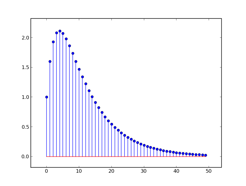
The overall response of this system is shown below:

\Delta + 0.9\mathcal{R}\Delta + 0.81\mathcal{R}^2\Delta + 0.729\mathcal{R}^3\Delta + 0.6561\mathcal{R}^3\Delta + \ldots

If traversing the cycle decreases or increases the magnitude of the signal, then the sample values will decay or grow, respectively, as time increases.

For the first system, the unit sample response is y[n] = (0.5)^ n; for the second, it's y[n] = (1.2)^ n. These system responses can be characterized by a single number, called the pole, which is the base of the geometric sequence. The value of the pole, p_0, determines the nature and rate of growth.

If p_0 \lt-1, the magnitude increases to infinity and the sign alternates.
If -1\lt p_0\lt 0, the magnitude decreases and the sign alternates.
If 0\lt p_0\lt 1, the magnitude decreases monotonically.
If p_0>1, the magnitude increases monotonically to infinity.

Any system for which the magnitude of the unit sample response increases to infinity, whether monotonically or not, is called unstable. Systems whose unit sample response decreases or stays constant in magnitude are called stable.

Because we are dealing with linear, time-invariant systems, these definitions hold not only for the unit sample response, but for the response of the system to any transient input (i.e., any input with finitely-many non-zero values).

1.6.2) Second-order systems

We will call these persistent long-term behaviors of a signal (and, hence, of the system that generates such signals) modes. For a fixed p_0, the first-order system only exhibited one mode (but different values of p_0 resulted in very different modes). As we build more complex systems, they will have multiple modes, which manifest as more complex behavior. Second-order systems are characterized by a system functional whose denominator polynomial is second order; they will generally exhibit two modes. We will find that it is the mode whose pole has the largest magnitude that governs the long-term behavior of the system. We will call this pole the dominant pole. Consider this system:

We can describe it with the operator equation

Y = 1.6\mathcal{R} Y - 0.63\mathcal{R}^2Y + X

so the system functional is

{\cal H} = \frac{1}{1 - 1.6 \mathcal{R} + 0.63 \mathcal{R}^2}

Here is its response to a unit sample signal:

We can try to understand its behavior by decomposing it in different ways. First, let's see if we can see it as a cascade of two systems. To do so, we need to find {\cal H}_1 and {\cal H}_2 such that {\cal H}_1 {\cal H}_2 = {\cal H}. We can do that by factoring {\cal H} to get

{\cal H}_1 = \frac{1}{1 - 0.7\mathcal{R}}~\text{and}~{\cal H}_2 = \frac{1}{1 - 0.9\mathcal{R}}

So, we have two equivalent version of this system, describable as cascades of two systems, one with p_0 = 0.9 and one with p_0 = 0.7:

This decomposition is interesting, but it does not yet let us understand the behavior of the system as the combination of the behaviors of two subsystems.

1.6.2.1) Additive decomposition

Another way to try to decompose the system is as the sum of two simpler systems. In this case, we seek {\cal H}_1 and {\cal H}_2 such that {\cal H}_1 + {\cal H}_2 = {\cal H}. We can do a partial fraction decomposition (don't worry if you don't remember the process for doing this...we won't need to solve problems like this in detail). We start by factoring, as above, and then figure out how to decompose into additive terms:

\begin{align} {\cal H} & = \frac{1}{1 - 1.6 \mathcal{R} + 0.63 \mathcal{R}^2}\\ & = \frac{1}{(1 - 0.9 \mathcal{R})(1 - 0.7\mathcal{R})}\\ & = \frac{A}{1 -0.9 \mathcal{R}} + \frac{B}{1 -0.7\mathcal{R}}\\ & = {\cal H}_1 + {\cal H}_2 \\ \end{align}

To find values for A and B, we start with

\frac{1}{(1 - 0.9 \mathcal{R})(1-0.7\mathcal{R})} = \frac{A}{1 -0.9 \mathcal{R}} + \frac{B}{1 -0.7\mathcal{R}}

multiply through by 1 - 1.6 \mathcal{R} + 0.63 \mathcal{R}^2 to get

1 = A(1-0.7\mathcal{R}) + B(1 - 0.9\mathcal{R})

and collect like terms:

1 = (A + B) - (0.7 A + 0.9 B) \mathcal{R}

Equating the terms that involve equal powers of \mathcal{R} (including constants as terms that involve \mathcal{R}^0), we have:

\begin{align} 1 & = A + B \\ 0 & = 0.7 A + 0.9 B \\ \end{align}

Solving, we find A = 4.5 and B = -3.5, so

\frac{Y}{X} = \frac{4.5}{1 -0.9 \mathcal{R}} + \frac{-3.5}{1 -0.7\mathcal{R}}

where

{\cal H}_1 = \frac{4.5}{1 - 0.9 \mathcal{R}}~\text{and}~{\cal H}_2 = \frac{-3.5}{1 - 0.7\mathcal{R}}

Check Yourself 6:

Verify that {\cal H}_1 + {\cal H}_2 = {\cal H}.

Here is (yet another) equivalent block diagram for this system, highlighting its decomposition into a sum:

We can understand this by looking at the responses of {\cal H}_1 and of {\cal H}_2 to the unit sample, and then summing them to recover the response of H to the unit sample. In the next figure, the blue stem plot is the overall signal, which is the sum of the green and red signals, which correspond to the top and bottom parts of the diagram, respectively.

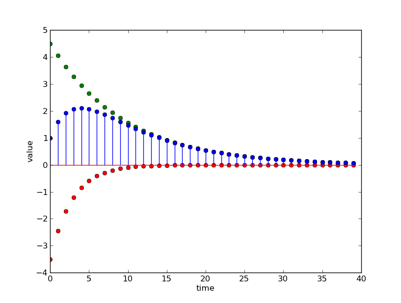
In this case, both of the poles (0.9 and 0.7) are less than 1, so the magnitude of the responses they generate decreases monotonically; their sum does not behave monotonically, but there is a time step at which the dominant pole completely dominates the other one, and the convergence is monotonic after that. If, instead, we had a system with system functional

{\cal H} = \frac{Y}{X} = \frac{1}{1 - 1.1 \mathcal{R}} + \frac{20}{1 - 0.9 \mathcal{R}}

what would the unit-sample response be? The first mode (first term of the sum) has pole 1.1, which means it will generate monotonically increasing output values. The second mode has pole 0.9, and will decrease monotonically. The plot below illustrates the sum of these two components:

The red points correspond to the output from the mode with pole 1.1; the green points correspond to the output from the mode with pole 0.9; and the blue stem plot shows the sum.

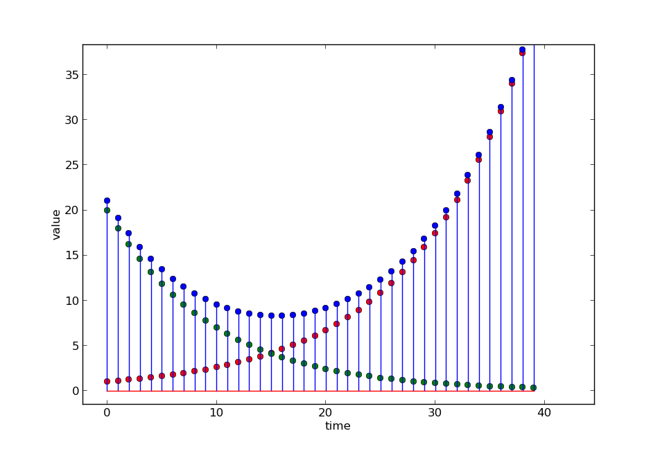
Here is a plot of the output of the system described by

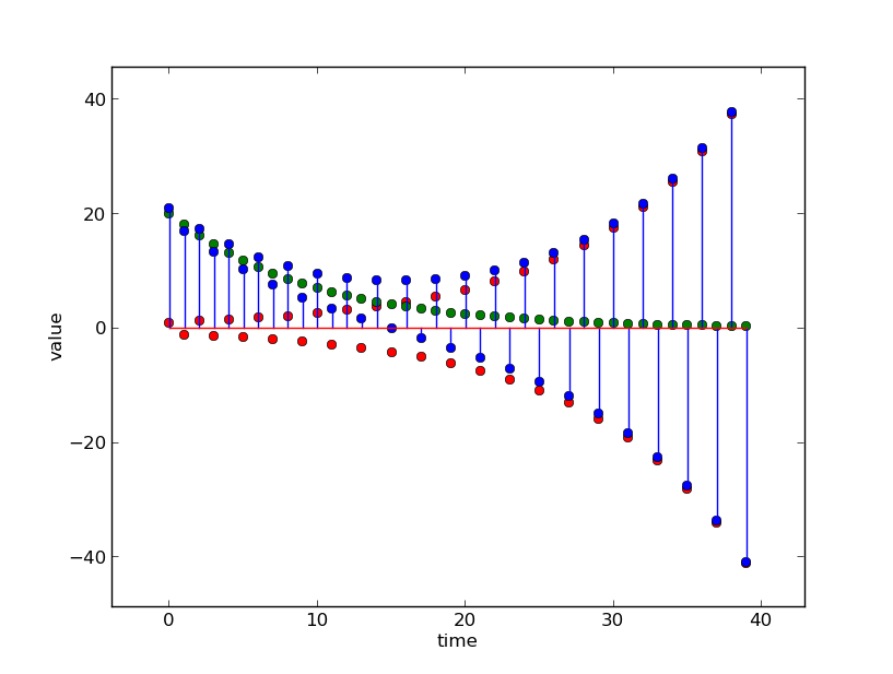
\frac{Y}{X} = \frac{21.1 \mathcal{R} + 21}{-0.99 \mathcal{R}^2 + 0.2 \mathcal{R} + 1}

It has poles 0.9 and -1.1.

The green dots are generated by the component with pole 0.9, the red dots are generated by the component with pole -1.1 and the blue dots are generated by the sum.

In these examples, as in the general case, the long-term unit-sample response of the entire system is governed by the unit-sample response of the mode whose pole has the larger magnitude. We call this pole the dominant pole. In the long run, the rate of growth of the exponential with the largest exponent will always dominate.

1.6.2.2) Complex poles

Consider a system described by the operator equation:

Y = 2 X + 2 \mathcal{R} X - 2\mathcal{R} Y - 4\mathcal{R}^2Y

It has system functional

\frac{Y}{X} = \frac{2 + 2\mathcal{R}}{1 + 2\mathcal{R} + 4\mathcal{R}^2}

But now, if we attempt to perform an additive decomposition on it, we find that the denominator cannot be factored to find real poles. Instead, we find that

\begin{align} \frac{Y}{X} & = \frac{2 + 2\mathcal{R}}{(1 - (-1 + \sqrt {-3})\mathcal{R})(1 - (-1 -\sqrt {-3})\mathcal{R})}\\ & \approx \frac{2 + 2\mathcal{R}}{(1 - (-1 + 1.732 j)\mathcal{R})(1 - (-1 -1.732 j)\mathcal{R})}\\ \end{align}

So, the poles are approximately -1 + 1.732 j and -1 - 1.732 j. Note that we are using j to signal the imaginary part of a complex number ³. What does that mean about the behavior of our system? Are the outputs real or complex? Do the output values grow or shrink with time? Difference equations that represent physical systems have real-valued coefficients. For instance, a bank account with interest \rho might be described with difference equation

y[n]=(1+\rho)y[n-1]+x[n]

The position of a robot moving toward a wall might be described with difference equation:

d_ o[n]=d_ o[n-1]+KTd_ o[n-2]-KTd_ i[n-1]

Difference equations with real-valued coefficients generate real-valued outputs from real-valued inputs. But, like the difference equation

y[n] = 2x[n] + 2x[n-1] - 2y[n-1] - 4y[n-1]

corresponding to system functional above, they might still have complex poles.

1.6.2.3) Polar representation of complex numbers

Sometimes it's easier to think about a complex number a + bj instead as r e^{j\Omega }, where

a = r \cos \Omega

b = r \sin \Omega

so that the magnitude, r, sometimes written as |a + bj|, is defined as

r = \sqrt {a^2 + b^2}

and the angle, \Omega, is defined as

\Omega = \tan ^{-1}(b, a)

So, if we think of (a, b) as a point in the complex plane, then (r, \Omega ) is its representation in polar coordinates.

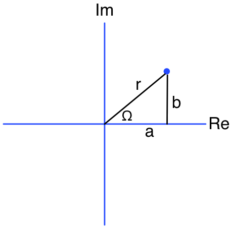
This representation is justified by Euler's equation $$e^{xj} = \cos x + j \sin x$$

which can be directly derived from series expansions of e^ z, \sin z and \cos z. To see that this is reasonable, let's take our number, represent it as a complex exponential, and then apply Euler's equation:

\begin{align} a + bj & = r e^{j\Omega }\\ & = r (\cos \Omega + j \sin \Omega )\\ & = \sqrt {a^2 + b^2} (\cos (\tan ^{-1}(b, a)) + j\sin (\tan ^{-1}(b, a)))\\ & = \sqrt {a^2 + b^2} (\frac{a}{\sqrt {a^2 + b^2}} + j \frac{b}{\sqrt {a^2 + b^2}}) \\ & = a + bj \\ \end{align}

Why should we bother with this change of representation? There are some operations on complex numbers that are much more straightforwardly done in the exponential representation. In particular, let's consider raising a complex number to a power. In the Cartesian representation, we get complex trigonometric polynomials. In the exponential representation, we get, in the quadratic case,

\begin{align} \left(r e^{j \Omega }\right)^2 & = r e^{j \Omega } r e^{j \Omega }\\ & = r^2 e^{j 2 \Omega }\\ \end{align}

More generally, we have that

\left(r e^{j\Omega }\right)^ n = r^ n e^{j n \Omega }

which is much tidier. This is an instance of an important trick in math and engineering: changing representations. We will often find that representing something in a different way will allow us to do some kinds of manipulations more easily. This is why we use diagrams, difference equations, operator equations and system functionals all to describe LTI systems. There is no one best representation; each has advantages under some circumstances (and disadvantages under others).

1.6.2.4) Complex modes

Now, we're equipped to understand how complex poles of a system generate behavior: they produce complex-valued modes. Remember that we can characterize the behavior of a mode as

{1\over 1-p\mathcal{R}}=1+p\mathcal{R}+p^2\mathcal{R}^2+\cdots +p^ n\mathcal{R}^ n+\cdots

For a complex pole p = re^{j\Omega }, p^ n = r^ n e^{j\Omega n}. So

{1\over 1-re^{j\Omega }\mathcal{R}}=1+re^{j\Omega }\mathcal{R}+r^2e^{j2\Omega }\mathcal{R}^2+\cdots

What happens as n tends to infinity when p is complex? Think of p^ n as a point in the complex plane with coordinates (r^ n, \Omega n). The radius, r^ n, will grow or shrink depending on the mode's magnitude, r. And the angle, \Omega n, will simply rotate, but will not affect the magnitude of the resulting value. Note that each new point in the sequence p^ n will be rotated by \Omega from the previous one. We will say that the period of the output signal is 2\pi / \Omega ; that is the number of samples required to move through 2 \pi radians (although this need not actually be an integer). The sequence spirals around the origin of the complex plane. Here is a case for r = 0.85, \Omega = \pi /4, that spirals inward, rotating \pi /4 radians on each step:

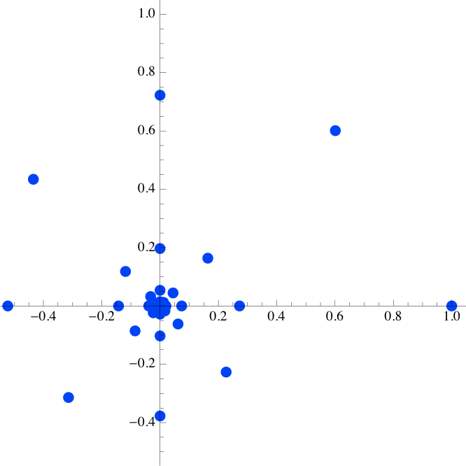
p = 0.85 e^{j \pi / 4} \approx 0.601 + 0.601 j

Here, for example, are plots of two other complex modes, with different magnitudes and rates of oscillation. In all cases, we are plotting the unit-sample response, so the first element in the series is the real value 1. The first signal clearly converges in magnitude to 0; the second one diverges (look carefully at the scales).

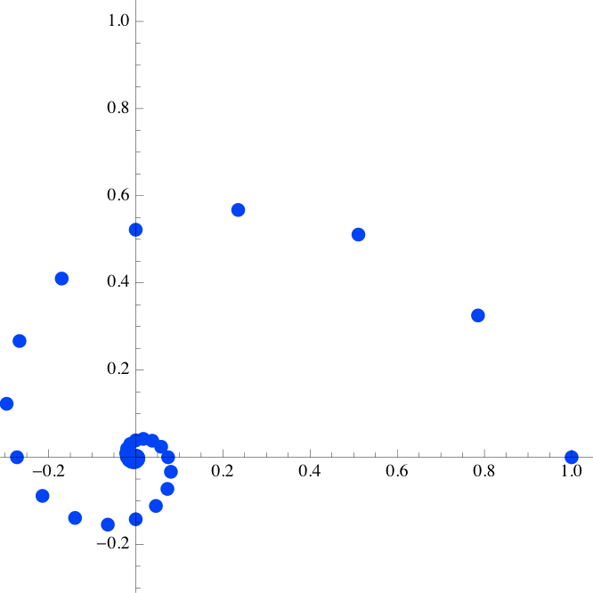
p = 0.85 e^{j \pi / 8} \approx 0.785 + 0.325 j

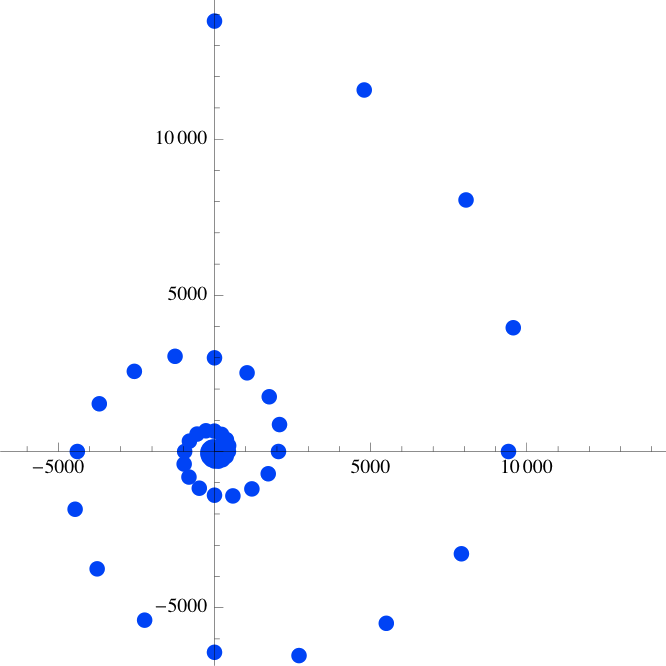
p = 1.1 e^{j \pi / 8} \approx 1.016 + 0.421 j

If complex modes occurred all by themselves, then our signals would have complex numbers in them. But isolated complex pole can result only from a difference equation with complex-valued coefficients. For example, to end up with this system functional

{Y\over X}={1\over 1-re^{j\Omega }\mathcal{R}}

we would need to have this difference equation, which has a complex coefficient.

y[n]-re^{j\Omega }y[n-1]=x[n]

But, we have difference equations with real parameters, so we can express the value of every sample of the output signal as a linear combination of inputs and previous values with real coefficients, so we know the output signal is real-valued at all samples. The reason this all works out is that, for polynomials with real coefficients, the complex poles always come in conjugate pairs: that is, pairs of complex numbers p = a + bj and p^* = a - bj. In the polar representation, the conjugate pair becomes

\begin{align} a \pm bj & = \sqrt {a^2 + b^2} e ^{j \tan ^{-1}(\pm b, a)}\\ & = \sqrt {a^2 + b^2} e^{\pm j \tan ^{-1}(b, a)} \\ \end{align}

where the only difference is in the sign of the angular part. If we look at a second-order system with complex-conjugate poles, the resulting polynomial has real-valued coefficients. To see this, consider a system with poles re^{j\Omega } and re^{-j\Omega }, so that

{Y\over X} = {1\over (1-re^{j\Omega }\mathcal{R})(1-re^{-j\Omega }\mathcal{R})}

Let's slowly multiply out the denominator:

\begin{align} (1-re^{j\Omega }\mathcal{R})(1-re^{-j\Omega }\mathcal{R}) & = 1 - re^{j\Omega }\mathcal{R} -re^{-j\Omega }\mathcal{R} + r^2e^{j\Omega }e^{-j\Omega }\mathcal{R}^2\\ & = 1 - r(e^{j\Omega } + e^{-j\Omega })\mathcal{R} + r^2e^{j\Omega -j\Omega }\mathcal{R}^2\\ \end{align}

Using the definition of the complex exponential e^{jx} = \cos x + j \sin x,

\begin{align} & = 1 - r(\cos \Omega + j\sin \Omega + \cos (-\Omega ) + j \sin (-\Omega ))\mathcal{R}+ r^2\mathcal{R}^2 \end{align}

Using trigonometric identities \sin -x = -\sin x and \cos -x =\cos x,

\begin{align} & = 1 - r(\cos \Omega + j\sin \Omega + \cos \Omega - j \sin \Omega )\mathcal{R} + r^2\mathcal{R}^2\\ & = 1 - 2 r\cos \Omega \mathcal{R} + r^2\mathcal{R}^2\\ \end{align}

So,

\frac{Y}{X} = \frac{1}{1 - 2 r\cos \Omega \mathcal{R} + r^2\mathcal{R}^2}

This is pretty cool! All of the imaginary parts cancel, and we are left with a system functional with only real coefficients, which corresponds to the difference equation

y[n] = x[n] + 2 r \cos \Omega y[n-1] - r^2 y[n-2]

1.6.2.5) Additive decomposition with complex poles

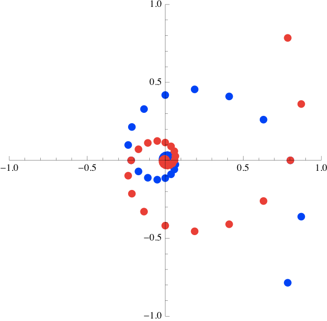
You can skip this section if you want to. To really understand these complex modes and how they combine to generate the output signal, we need to do an additive decomposition. That means doing a partial fraction expansion of

{Y\over X} = {1\over (1-re^{j\Omega }\mathcal{R})(1-re^{-j\Omega }\mathcal{R})}

It's a little trickier than before, because we have complex numbers, but the method is the same. The end result is that we can decompose this system additively to get

{Y\over X} = \frac{\frac{1}{2}(1 - j \cot \Omega )}{1-re^{j\Omega }\mathcal{R}} +\frac{\frac{1}{2}(1 + j \cot \Omega )}{1-re^{-j\Omega }\mathcal{R}}

What is the unit-sample response of each of these modes? What is the unit-sample response of their sum? This might be making you nervous...it's hard to see how everything is going to come out to be real in the end. But, let's examine the response of the additive decomposition; it's the sum of the outputs of the component systems. So, if x[n] =\delta [n] ,

\begin{align} y[n] & = \frac{1}{2}(1 - j \cot \Omega ) r^ n e^{jn\Omega } + \frac{1}{2}(1 + j \cot \Omega ) r^ n e^{-jn\Omega }\\ & = r^ n(\cos n \Omega + \cot \Omega \sin n \Omega )\\ \end{align}

which is entirely real. The figure below shows the modes for a system with poles 0.85 e^{j\pi / 8} and 0.85 e^{-j \pi / 8} : the blue series starts at \frac{1}{2}(1 - j\cot (\pi /8)) and traces out the unit sample response of the first component; the second red series starts at \frac{1}{2}(1 + j \cot (\pi /8)) and traces out the unit sample response of the second component.

Note that the imaginary parts of the contributions of each of the modes are qual but opposite in sign, and that the real parts are exactly equal. If we sum these components, the real part of the output is going to be twice the real part of these elements. The figure below shows the unit sample response of the entire system.

1.6.2.6) Importance of magnitude and period

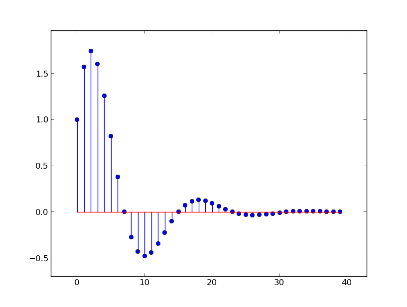
Both r and \Omega tells us something very useful about the way in which the system behaves. In the previous section, we derived an expression for the samples of the unit sample response for a system with a pair of complex poles. It has the form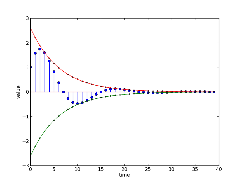

y[n] = r^ n(\cos n \Omega + \alpha \sin n \Omega )

where \alpha is a constant. We know that (\cos n \Omega + \alpha \sin n \Omega ) cannot possibly be less than -\sqrt {1 + \alpha ^2} or greater than \sqrt {1 + \alpha ^2}. These bounds provide an envelope that constrains where the values of the signal can be as a function of time, and help us understand the rate of growth or decay of the signal, as shown below. The red and green curves are \pm \sqrt {1 + \alpha ^2} r^ n, for a system where r = 0.85, \Omega = \pi / 8, and \alpha = 2.414.

The value of r governs the rate of exponential decrease. The value of \Omega governs the rate of oscillation of the curve. It will take 2 \pi / \Omega (the period of the oscillation) samples to go from peak to peak of the oscillation ⁴. In our example, \Omega = \pi / 8 so the period is 16; you should be able to count 16 samples from peak to peak.

1.6.2.7) Poles and behavior: summary

In a second-order system, if we let p_0 be the pole with the largest magnitude, then there is a time step at which the behavior of the dominant pole begins to dominate; after that time step

If p_0 is real and
- p_0\lt -1, the magnitude increases to infinity and the sign alternates.
- -1\lt p_0\lt 0, the magnitude decreases and the sign alternates.
- 0\lt p_0\lt 1, the magnitude decreases monotonically.
- p_0\gt 1, the magnitude increases monotonically to infinity.
If p_0 is complex and \Omega is its angle, then the signal will be periodic, with period 2 \pi / \Omega .
If p_0 is complex
- and |p_0| \lt 1, the amplitude of the response decays to 0.
- and |p_0| \gt 1, the amplitude of the response increases to infinity.

Remember that any system for which the output magnitude increases to infinity, whether monotonically or not, is called unstable. Systems whose output magnitude decreases or stays constant are called stable. As we have seen in our examples, when we add multiple modes, it is the mode with the largest pole, that is, the dominant pole that governs the long-term behavior.

1.6.3) Higher-order systems

Recall that we can describe any system in terms of a system functional that is the ratio of two polynomials in \mathcal{R} (and assuming a_0 = 1):

{Y\over X}={b_0+b_1\mathcal{R}+b_2\mathcal{R}^2+b_3\mathcal{R}^3+\cdots \over 1+a_1\mathcal{R}+a_2\mathcal{R}^2+a_3\mathcal{R}^3+\cdots }

Regrouping terms, we can write this as the operator equation:

Y = (b_0+b_1\mathcal{R}+b_2\mathcal{R}^2+b_3\mathcal{R}^3+\cdots )X - (a_1\mathcal{R}+a_2\mathcal{R}^2+a_3\mathcal{R}^3+\cdots )Y

and construct an equivalent block diagram:

Returning to the general polynomial ratio

{Y\over X}={b_0+b_1\mathcal{R}+b_2\mathcal{R}^2+b_3\mathcal{R}^3+\cdots \over 1+a_1\mathcal{R}+a_2\mathcal{R}^2+a_3\mathcal{R}^3+\cdots }

We can factor the denominator of an n th-order polynomial into n factors, and then perform a partial fraction expansion, to turn it into the form of a sum of terms. We won't go over the details here (there are nice tutorials online), but it comes out in the form:

{Y\over X}={C_0\over 1-p_0\mathcal{R}}+{C_1\over 1-p_1\mathcal{R}}+{C_2\over 1-p_2\mathcal{R}}+\cdots +D_0+D_1\mathcal{R}+D_2\mathcal{R}^2+\cdots

where the C_ k and D_ k are constants defined in terms of the a_ i and b_ j from the original polynomial ratio. It's actually a little bit trickier than this: if there are complex poles, then for each conjugate pair of complex poles, we would put in a second-order system with real coefficients that expresses the contribution of the sum of the complex modes. The constant term D_0 and the terms with \mathcal{R}^ k in the numerator occur if the numerator has equal or higher order than the denominator. They do not involve feedback and don't affect the long-term behavior of the system. One mode of the form p_ i^ n arises from each factor of the denominator. This modal decomposition leads us to an alternative block diagram:

We can fairly easily observe that the behavior is going to be the sum of the behaviors of the individual modes, and that, as in the second-order case, the mode whose pole has the largest magnitude will govern the qualitative long-term nature of the behavior of the system in response to a unit-sample input.

1.6.4) Finding poles

In general, we will find that if the denominator of the system functional {\cal H} is a k th order polynomial, then it can be factored into the form (1 - p_0\mathcal{R})(1 - p_1\mathcal{R})\ldots (1 - p_{k-1}\mathcal{R}). We will call the p_ i values the poles of the system. The entire persistent output of the system can be expressed as a scaled sum of the signals arising from each of these individual poles. We're doing something interesting here! We are using the PCAP system backwards for analysis. We have a complex thing that is hard to understand monolithically, so we are taking it apart into simpler pieces that we do understand. It might seem like factoring polynomials in this way is tricky, but there is a straightforward way to find the poles of a system given its denominator polynomial in \mathcal{R}. We'll start with an example. Assume the denominator is 12\mathcal{R}^2 - 7 \mathcal{R} + 1. If we play a quick trick, and introduce a new variable z = 1 / \mathcal{R}, then our denominator becomes

\frac{12}{z^2} - \frac{7}{z} + 1

We'd like to find the roots of this polynomial, which, if you multiply through by z^2, is equivalent to finding the roots of this poyinomial:

12 - 7z + z^2 = 0

The roots are 3 and 4. If we go back to our original polynomial in \mathcal{R}, we can see that:

12\mathcal{R}^2 - 7 \mathcal{R} + 1 = (1 - 4\mathcal{R}) (1 - 3\mathcal{R})

so that our poles are 4 and 3. So, remember, the poles are not the roots of the polynomial in \mathcal{R}, but are the roots of the polynomial in the reciprocal of \mathcal{R}. The roots of a polynomial can be a combination of real and complex numbers, with the requirement that if a complex number p is a root, then so is its complex conjugate, p^*.

1.6.4.1) Pole-Zero cancellation

For some systems, we may find that it is possible to cancel matching factors from the numerator and denominator of the system functional. If the factors represent poles that are not at zero, then although it may be theoretically supportable to cancel them, it is unlikely that they would match exactly in a real system. If we were to cancel them in that case, we might end up with a system model that was a particularly poor match for reality ⁵. So, we will only consider canceling poles and zeros at zero. In this example:

{\cal H} = \frac{\mathcal{R}}{\mathcal{R} - 1.6 \mathcal{R}^2 + 0.63 \mathcal{R}^3}

we can cancel \mathcal{R}, getting

{\cal H} = \frac{1}{1 - 1.6 \mathcal{R} + 0.63 \mathcal{R}^2}

Now, we find the poles by finding the roots of the equation

z^2 - 1.6 z + 0.63 = 0

1.6.4.2) Repeated roots

In some cases, the equation in z will have repeated roots. For example, z^2 - z + 0.25, which has two roots at 0.5. In this case, the system has a repeated pole; it is still possible to perform an additive decomposition, but it is somewhat trickier. Ultimately, however, it is still the magnitude of the largest root that governs the long-term convergence properties of the system.

1.6.5) Superposition

The principle of superposition states that the response of a LTI system to a sum of input signals is the sum of the responses of that system to the components of the input. So, given a system with system functional {\cal H}, and input X = X_1 + X_2,

Y = {\cal H} X = {\cal H} (X_1 + X_2) = {\cal H} X_1 + {\cal H} X_2

So, although we have been concentrating on the unit sample response of systems, we can see that, to find the response of a system to any finite signal, we must simply sum the responses to each of the components of that signal; and those responses will simply be scaled, delayed copies of the response to the unit sample. If \Phi is a polynomial in \mathcal{R} and X = \Phi \Delta , then we can use what we know about the algebra of polynomials in \mathcal{R} (remembering that {\cal H} is a ratio of polynomials in \mathcal{R}) to determine that

Y = {\cal H}X = {\cal H} (\Phi \Delta ) = \Phi ({\cal H} \Delta )

So, for example, if X = (-3\mathcal{R}^2 + 20\mathcal{R}^4)\Delta , then Y = {\cal H}X = {\cal H}(-3\mathcal{R}^2 + 20 \mathcal{R}^4)\Delta = (-3\mathcal{R}^2 +20\mathcal{R}^4){\cal H}\Delta. From this equation, it is easy to see that once we understand the unit-sample response of a system, we can see how it will respond to any finite input. We might be interested in understanding how a system {\cal H} responds to a step input signal. Let's just consider the basic step signal, U, defined as u[n]=1 if n = 0 and 0 if otherwise.

We can express U as an infinite sum of increasingly delayed unit-sample signals:

\begin{align} U & = \Delta + \mathcal{R} \Delta + \mathcal{R}^2 \Delta + \mathcal{R}^3 \Delta + \cdots\\ & = (1 + \mathcal{R} + \mathcal{R}^2 + \mathcal{R}^3 + \cdots ) \Delta\\ \end{align}

The response of a system to U will therefore be an infinite sum of unit-sample responses. Let Z = {\cal H} \Delta be the unit-sample response of {\cal H}.

Then:

\begin{align} {\cal H} U & = {\cal H} (1 + \mathcal{R} + \mathcal{R}^2 + \mathcal{R}^3 + \cdots ) \Delta\\ & = (1 + \mathcal{R} + \mathcal{R}^2 + \mathcal{R}^3 + \cdots ) H \Delta\\ & = (1 + \mathcal{R} + \mathcal{R}^2 + \mathcal{R}^3 + \cdots ) Z\\ \end{align}

Let's consider the case where {\cal H} is a first-order system with a pole at p. Then,

z[n] = p^ n

If Y = {\cal H} U, then

\begin{align} y[n] & = z[n] + z[n-1] + z[n-2] + \cdots + z[0]\\ & = \sum _{k = 0}^ n z[k]\\ & = \sum _{k = 0}^ n p^ k\\ \end{align}

It's clear that, if |p| \gt = 1 then y[n] will grow without bound; but if 0 \lt p \lt 1 then, as n goes to infinity, y[n] will converge to 1 / (1 - p). We won't study this in any further detail, but it's useful to understand that the basis of our analysis of systems applies very broadly across LTI systems and inputs.

1.7) Summary of system behavior

Here is some terminology that will help us characterize the long-term behavior of systems.

A signal is transient if it has finitely many non-zero samples. Otherwise, it is persistent.
A signal is bounded if there is exist upper and lower bound values such that the samples of the signal never exceed those bounds; item otherwise it is unbounded.

Now, using those terms, here is what we can say about system behavior:

A transient input to an acyclic (feed-forward) system results in a transient output.
A transient input to a cyclic (feed-back) system results in a persistent output.
The poles of a system are the roots of the denominator polynomial of the system functional written in terms of z = 1/\mathcal{R}.
The dominant pole is the pole with the largest magnitude.
If the dominant pole has magnitude \gt 1, then in response to a bounded input, the output signal will be unbounded.
If the dominant pole has magnitude \lt 1, then in response to a bounded input, the output signal will be bounded; in response to a transient input, the output signal will converge to 0.
If the dominant pole has magnitude 1, then in response to a bounded input, the output signal will be bounded; in response to a transient input, it will converge to some constant value.
If the dominant pole is real and positive, then in response to a transient input, the signal will, after finitely many steps, begin to increase or decrease monotonically.
If the dominant pole is real and negative, then in response to a transient input, the signal will, after finitely many steps, begin to alternate signs (or, to say it another way, the signal will start to oscillate with a period of 2 timesteps).
If the dominant pole is complex, then in response to a transient input, the signal will, after finitely many steps, begin to be periodic, with a period of 2 \pi / \Omega , where \Omega is the 'angle' of the pole.

Footnotes

¹There are always unimportant outputs, and which outputs we care about depend on the system we are desigining or analyzing. Think about the number of moving parts in a car; they are not all important for steering! (click to return to text)

²Note that \delta is the lowercase version of \Delta, both of which are the Greek letter "delta." (click to return to text)

³We use j instead of i because, to an electrical engineer, i stands for current, and cannot be re-used! (click to return to text)

⁴We are being informal here, in two ways. First, the signal does not technically have a period, because unless r=1, it doesn't return to the same point. Second, unless r=1, then distance from peak to peak is not exactly 2\pi / \Omega; however, for most signals, it will give a good basis for estimating \Omega (click to return to text)

⁵Don't worry too much if this doesn't make sense to you. Take 6.003 and/or 6.302 to learn more! (click to return to text)