6.01 Course Notes
6) Search
Table of Contents
- 6) Search
- 6.1) Introduction
- 6.2) State-space Search
- 6.3) Search Algorithms
- 6.3.1) Basic Search
- 6.3.2) Basic Pruning
- 6.3.3) Stacks and Queues
- 6.3.4) Depth-First Search (DFS)
- 6.3.5) Breadth-First Search (BFS)
- 6.3.6) Dynamic Programming
- 6.4) Example: Numeric Search Domain
- 6.5) Computational complexity
- 6.6) Uniform cost search
- 6.7) Search with heuristics
6.1) Introduction
For many real-world problems, finding a solution analytically is either difficult or impossible. In this chapter, we will examine algorithms that allow us to solve a large class of problems by taking advantage of the speed and memory of computers, and to guarantee that the solutions generated are optimal in some way.
One example of this kind of problem is finding a path through a maze. Another example is plotting a route from a starting point on a map to a goal point.
We will develop a systematic approach to solving such problems by formulating them as instances of a graph search (or a "state-space search") problem, for which there are simple algorithms that perform well.
In the lab exercises of this course, we have implemented several brains for our robots. We used wall-following to navigate through the world and we used various linear controllers to drive down the hall and to control the robot head. In the first case, we just wrote a program that we hoped would do a good job. When we were studying linear controllers, we, as designers, made models of the controller's behavior in the world and tried to prove whether it would behave in the way we wanted it to, taking into account a longer-term pattern of behavior.
Often, we will want a system to generate complex long-term patterns of behavior, but we will not be able to write a simple control rule to generate those behavior patterns. In that case, we'd like the system to evaluate alternatives for itself, but instead of evaluating single actions, it will have to evaluate whole sequences of actions, deciding whether they're a good thing to do given the current state of the world.
Let's think of the problem of navigating through a city, given a road map, and knowing where we are. We can't usually decide whether to turn left at the next intersection without deciding on a whole path.
As always, the first step in the process will be to come up with a formal model of a real-world problem that abstracts away the irrelevant detail. So, what, exactly, is a path? The car we're driving will actually follow a trajectory through continuous space(time), but if we tried to plan at that level of detail we would fail miserably. Why? First, because the space of possible trajectories through two-dimensional space is just too enormous. Second, because when we're trying to decide which roads to take, we don't have the information about where the other cars will be on those roads, which will end up having a huge effect on the detailed trajectory we'll end up taking.
So, we can divide the problem into two levels: planning in advance which turns we'll make at which intersections, but deciding 'on-line', while we're driving, exactly how to control the steering wheel and the gas to best move from intersection to intersection, given the current circumstances (other cars, stop-lights, etc.).
We can make an abstraction of the driving problem to include road intersections and the way they're connected by roads. Then, given a start and a goal intersection, we could consider all possible paths between them, and choose the one that is best.
What criteria might we use to evaluate a path? There are all sorts of reasonable ones: distance, time, gas mileage, traffic-related frustration, scenery, etc. Generally speaking, the approach we'll outline below can be extended to any criterion that is additive: that is, your happiness with the whole path is the sum of your happiness with each of the segments. We'll start with the simple criterion of wanting to find a path with the fewest "steps"; in this case, it will be the path that traverses the fewest intersections. Then we will generalize our methods to handle problems where different actions have different costs.
One possible algorithm for deciding on the best path through a map of the road intersections in this (very small) world
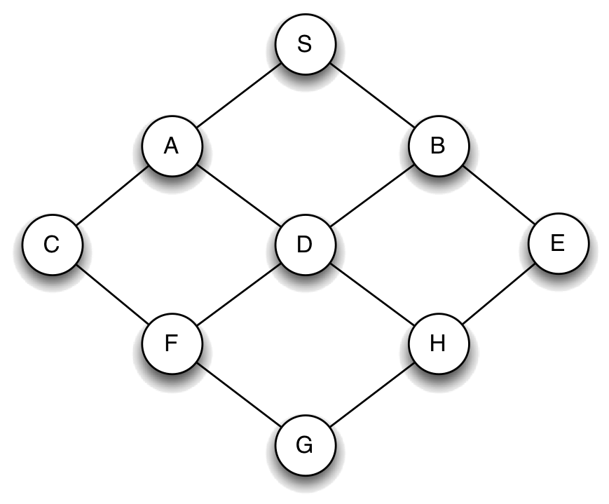
We can get a much better handle on this problem, by formulating it as an instance of a graph search (or a "state-space search") problem, for which there are simple algorithms that perform well.
6.2) State-space Search
To completely specify a state-space search problem, we need:
- a (possibly infinite) set of states in which the underlying system can be in;
- a starting state, which is an element of the set of states;
- a goal test, which is a procedure that can be applied to any state, and returns True if that state can serve as a goal; 1
- a means of determining a state's successors, which are all possible states that can be reached from a given state.
The decision about what constitutes a state is a modeling decision, and depends heavily on the problem we are trying to solve. In the grid example, a state might be a tuple (x,y). In the map example, a state might be an intersection or an address. We will also see examples where the state is an integer or a string or a list or other object.
When all of the information is put together, we can think of this model as specifying a labeled graph (in the computer scientist's sense), in which the states are the vertices, and the edges represent a transition from one state to another.
Let's consider a search in the following small city:

For this city, we might make a model in which
- The set of states is the intersections {'S', 'A', 'B', 'C', 'D', 'E', 'F', 'G', 'H'}
- The starting state is 'S'.
- The goal test is something like: lambda state: state == 'H'
Each state's successors are represented by a successors function, such as lambda s: map[s] where map is the following dictionary:
{'S' : ['A', 'B'],
'A' : ['S', 'C', 'D'],
'B' : ['S', 'D', 'E'],
'C' : ['A', 'F'],
'D' : ['A', 'B', 'F', 'H'],
'E' : ['B', 'H'],
'F' : ['C', 'D', 'G'],
'H' : ['D', 'E', 'G'],
'G' : ['F', 'H']}
where each key is a state, and its value is a list of states that can be reached from it in one step. 2
We can think of this structure as defining a search tree, like this:
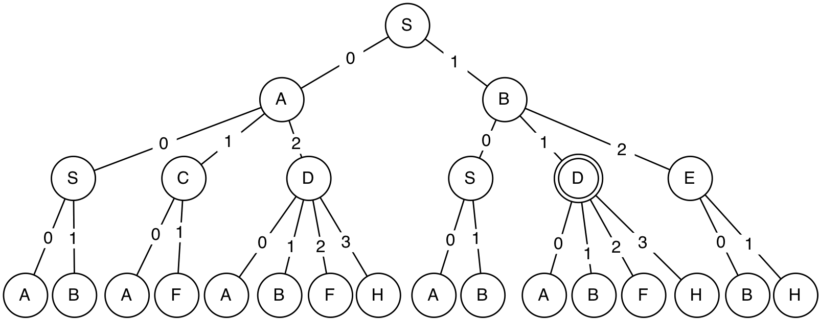
It has the starting state, S, at the root node, and then each node has its neighboring states as children. Layer k of this tree contains all possible paths of length k through the graph.
6.2.1) Representing search trees
We will need a way to represent the tree as a Python data structure as we construct it during the search process. We will start by defining a class to represent a search node, which is one of the circles in the tree.
Each search node must contain:
- the state of the node
- the node's parent (search node from which this node was reached)
Note that states and nodes are not the same thing! In this tree, there are many nodes labeled by the same state; they represent different paths to and through the state. This is an important distinction: we can think of a node as representing a path from the starting state to some other state.
Here is a Python class representing a search node. It's pretty straightforward.
class SearchNode:
    def __init__(self,state,parent):
        self.state = state
        self.parent = parent

    def path(self):
        if self.parent == None:
            return [self.state]
        else:
            return self.parent.path() + [self.state]
Note that the path method will return a list of the states contained in the path
represented by this node, starting with the root's state, and ending with this
node's state.
The path corresponding to our double-circled node is ['S', 'B', 'D'].
6.3) Search Algorithms
One way to really "brute-force" our way to a solution to this problem would be to perform what is called a "British Museum" search: we could systematically create the tree containing all possible paths beginning with the start node, and then look through all of these paths to find a solution that is somehow optimal.
However, this method is problematic in more ways than one. We will find that, with this approach, we will waste a lot of time expanding paths that don't make any sense (for example, a path S\rightarrow A\rightarrow S\rightarrow A\rightarrow \ldots ). More glaringly, there could be infinitely many paths! So we could spend an eternity trying to build the tree, without ever actually starting to look for out optimal path. It turns out that, due to the nature of these problems, we will be able to build the tree and search for a solution simultaneously.
Throughout this chapter, we will describe a sequence of search algorithms of increasing sophistication and efficiency. An ideal algorithm will take a problem description as input and return a path from the start to a goal state if one exists, and return None if no such path exists.
6.3.1) Basic Search
How can we systematically search for a path to the goal? There are (at least) two plausible strategies:
- Start down a path, keep trying to extend it until you get stuck, and then go back to the last choice you had, and go a different way. This is how kids often solve mazes on restaurant placemats. We'll call it depth-first search.
- Go layer by layer through the tree, first considering all paths of length 1, then all of length 2, etc. We'll call this breadth-first search.
Both of the search strategies described above can be implemented using a procedure with this basic structure (represented in pseudocode)3:
def search(successors, start_state, goal_test):
    if the start_state satisfies the goal_test condition:
        return a path containing only the start_state

    initialize an empty agenda of nodes we wish to search eventually
    add a SearchNode representing the start_state, with no parent, to the agenda

    while the agenda is nonempty:
        pull a node off of the agenda
        for each child state reachable from this node's state:
            if the child state satisfies the goal_test condition:
                return the path from the starting state to the child's state
            else:
                make a child node with current node as parent
                add the child node to the agenda

    no path from start to goal; return None
We start by checking to see if the initial state is a goal state. If so, we just return a path consisting of the initial state.
Otherwise, we have real work to do. We create a SearchNode representing a path with just the initial state; we take this node to be the root node of the search tree.
During the process of constructing the search tree, we will use a data structure, called an agenda, to keep track of which nodes in the partially constructed tree are on the fringe, ready to be expanded, by adding their children to the tree. We initialize the agenda to contain the root node. Now, we enter a loop that will run until the agenda is empty (we have no more paths to consider), but could stop sooner.
Inside the loop, we select a node from the agenda (more on how we decide which one to take out in a bit) and expand it. To expand a node we call the successors function on the node's state and visit the successor states.
When we visit a state, we check to see if it satisfies the goal test. If it does, we're done! We return the path leading to that state.
If this state it doesn't satisfy the goal test, then we add the new node to the agenda. We continue this process until we find a goal state or the agenda becomes empty. This is not quite yet an algorithm, though, because we haven't said anything about what it means to add and extract nodes from the agenda. And, we'll find that it will do some very stupid things, in its current form.
We'll start by curing the stupidities, and then return to the question of how best to select nodes from the agenda.
6.3.2) Basic Pruning
As we mentioned before, if you examine the full search tree, you can see that some of the paths it contains are completely ridiculous. It can never be reasonable, if we're trying to find the shortest path between two states, to go back to a state we have previously visited on that same path. So, to avoid trivial infinite loops, we can adopt the following rule:
If we can apply this rule, then we will be able to remove a number of branches from the tree, as shown here:
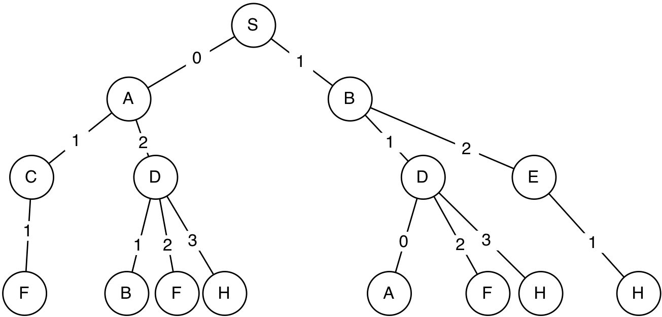
It is relatively straightforward to modify our pseudocode to implement this rule: before adding a new path to the agenda, check whether its end state already appears in the path, and, if so, do not add it to the agenda.
The next pruning rule doesn't make a difference in the current domain, but can have a big effect in other domains:
To handle this in the code, we have to keep track of which new states we have reached in expanding this node, and if we find another way to reach one of those states, we just ignore it.
Now, we have to think about how to extract nodes from the agenda.
6.3.3) Stacks and Queues
In designing algorithms, we frequently make use of two simple data structures: stacks and queues. You can think of them both as abstract data types that support two operations: push and pop. The push operation adds an element to the stack or queue, and the pop operation removes an element. The difference between a stack and a queue is what element you get back when you do a pop.
- stack: When you pop a stack, you get back the element in the stack that was added most recently. A stack is also called a LIFO, for last in, first out.
- queue: When you pop a queue, you get back the element in the queue that you added earliest. A queue is also called a FIFO, for first in, first out.
In Python, we can use lists to represent both stacks and queues. If data is a list, then data.pop(0) removes the first element from the list and returns it, and data.pop(-1) removes the last element and returns it.
Here is a class representing stacks as lists. It always adds new elements to the end of the list, and pops items off of the same end, ensuring that the most recent items get popped off first.
class Stack:
    def __init__(self):
        self.data = []
    def push(self, item):
        self.data.append(item)
    def pop(self):
        return self.data.pop()
    def is_empty(self):
        return len(self.data) == 0
Here is a class representing queues as lists. It always adds new elements to the end of the list, and pops items off of the front, ensuring that the oldest items get popped off first.
class Queue:
    def __init__(self):
        self.data = []
    def push(self, item):
        self.data.append(item)
    def pop(self):
        return self.data.pop(0)
    def is_empty(self):
        return len(self.data) == 0
We will use stacks and queues to implement our search algorithms, but it is important to note that they could just as easily be implemented using lists instead of these wrapper classes.
6.3.4) Depth-First Search (DFS)
Now we can easily describe depth-first search by saying that it's an instance of the generic search procedure described above, but in which the agenda is a stack: that is, we always expand the node we most recently put into the agenda.
The code listing below shows our implementation of depth-first search. Text in red represents code specific to DFS. successors is a function takes a state and returns a list of states reachable from that state (in one step), start_state is a state and goal_test is a function that takes a state and returns True if that state satisfies the goal condition and False otherwise.
def depth_first_search(successors, start_state, goal_test):
    if goal_test(start_state):
        return [start_state]
    start_node = SearchNode(start_state, None)
    agenda = Stack()
    agenda.push(start_node)
    while not agenda.is_empty():
        parent = agenda.pop()
        new_child_states = [] #for pruning rule 2
        for child_state in successors(parent.state):
            child = SearchNode(child_state, parent)
            if goal_test(child_state):
                return child.path()
            elif child_state in new_child_states: #pruning rule 2
                pass
            elif child_state in parent.path(): #pruning rule 1
                pass
            else:
                new_child_states.append(child_state)
                agenda.push(child)
    return None
You can see several operations on the agenda. We:
- Create an empty Stack instance, and let that be the agenda.
- Push the initial node onto the agenda.
- Test to see if the agenda is empty.
- Pop the node to be expanded off of the agenda.
- Push newly visited nodes onto the agenda.
Because the agenda is an instance of the Stack class, subsequent operations on the agenda ensure that it will act like a stack, and guarantee that children of the most recently expanded node will be chosen for expansion next.
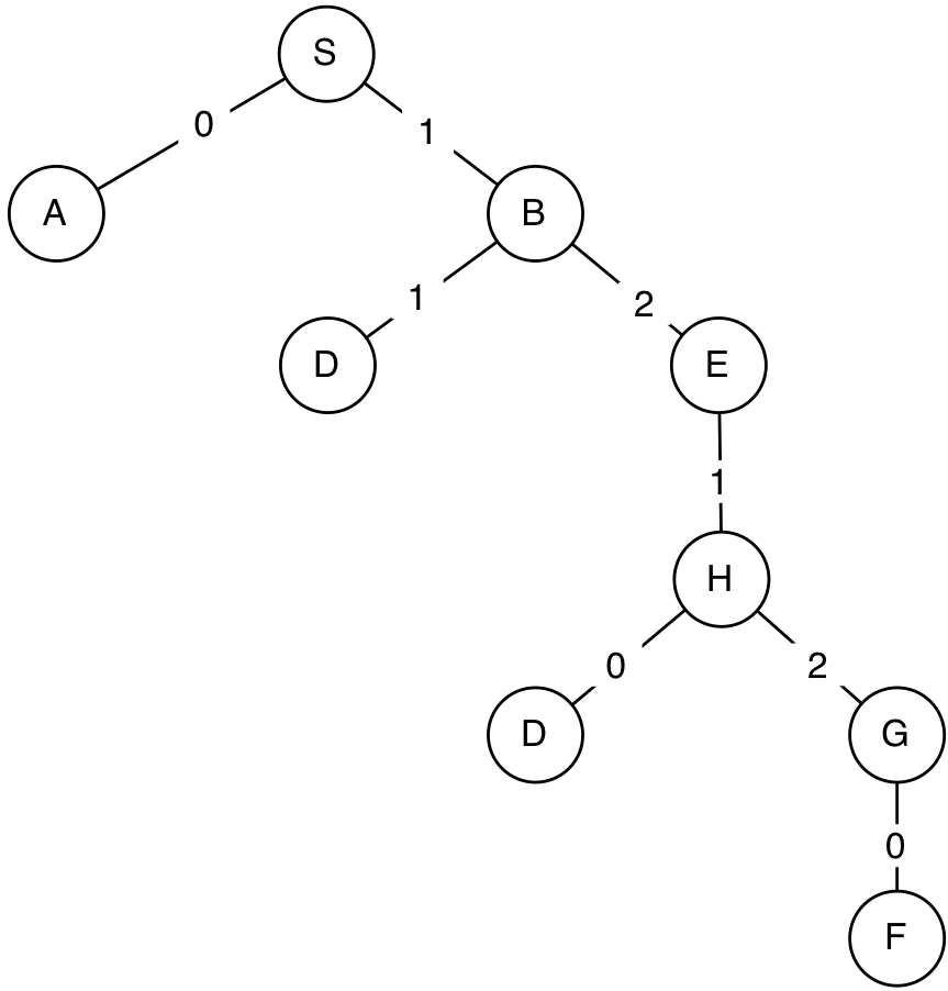
So, let's see how this search method behaves on our city map, with start state S and goal state F. Here is a trace of the algorithm:
agenda:  Stack([S])
   expanding:  S
agenda:  Stack([S->A, S->B])
   expanding:  S->B
agenda:  Stack([S->A, S->B->D, S->B->E])
   expanding:  S->B->E
agenda:  Stack([S->A, S->B->D, S->B->E->H])
   expanding:  S->B->E->H
agenda:  Stack([S->A, S->B->D, S->B->E->H->D, S->B->E->H->G])
   expanding:  S->B->E->H->G
8  states visited
Final path: ['S', 'B', 'E', 'H', 'G', 'F']
You can see that in this world, the search never needs to "backtrack", that is, to go back and try expanding an older path on its agenda. It is always able to push the current path forward until it reaches the goal. Here is the search tree generated during the depth-first search process.
Here is another city map (it's a weird city, we know, but maybe a bit like trying to drive in Boston):
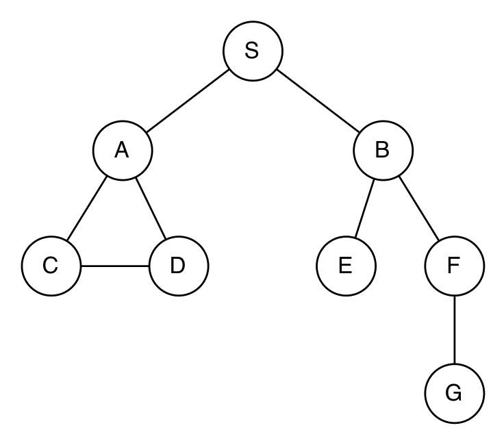
In this city, depth-first search behaves a bit differently (trying to go from S to D this time):
agenda:  Stack([S])
   expanding:  S
agenda:  Stack([S->A, S->B])
   expanding:  S->B
agenda:  Stack([S->A, S->B->E, S->B->F])
   expanding:  S->B->F
agenda:  Stack([S->A, S->B->E, S->B->F->G])
   expanding:  S->B->F->G
agenda:  Stack([S->A, S->B->E])
   expanding:  S->B->E
agenda:  Stack([S->A])
   expanding:  S->A
7  states visited
Final path: ['S', 'A', 'D']
In this case, it explores all possible paths down in the right branch of the world, and then has to backtrack up and over to the left branch.
Here are some important properties of depth-first search:
- It may run forever if we don't apply pruning rule 1, potentially going back and forth from one state to another, forever.
- It may run forever in an infinite domain (as long as the path it's on has a new child that hasn't been previously visited, it can go down that path forever; we'll see an example of this in the last section).
- It doesn't necessarily find the shortest path (as we can see from the very first example), though is guaranteed to find a path if one exists (and the search space is finite).
- It is generally efficient in the amount of space it requires to store the agenda, which will be a constant factor times the depth of the path it is currently considering (we'll explore this in more detail in the section on complexity.
6.3.5) Breadth-First Search (BFS)
To change to breadth-first search, we need to choose the oldest, rather than the newest paths from the agenda to expand. All we have to do is change the agenda to be a queue instead of a stack, and everything else stays the same, in the code.
def breadth_first_search(successors, start_state, goal_test):
    if goal_test(start_state):
        return [start_state]
    start_node = SearchNode(start_state, None)
    agenda = Queue()
    agenda.push(start_node)
    while not agenda.is_empty():
        parent = agenda.pop()
        new_child_states = [] #for pruning rule 2
        for child_state in successors(parent.state):
            child = SearchNode(child_state, parent)
            if goal_test(child_state):
                return child.path()
            elif child_state in new_child_states: #pruning rule 2
                pass
            elif child_state in parent.path(): #pruning rule 1
                pass
            else:
                new_child_states.append(childState)
                agenda.push(child)
    return None
Here is how breadth-first search works, looking for a path from S to F in our first city:
agenda:  Queue([S])
   expanding:  S
agenda:  Queue([S->A, S->B])
   expanding:  S->A
agenda:  Queue([S->B, S->A->C, S->A->D])
   expanding:  S->B
agenda:  Queue([S->A->C, S->A->D, S->B->D, S->B->E])
   expanding:  S->A->C
7  states visited
Final path: ['S', 'A', 'C', 'F']
We can see it proceeding systematically through paths of length two, then length three, finding the goal among the length-three paths. Note also that this is shorter than the path found by DFS!
Here are some important properties of breadth-first search:
- It always returns a shortest (least number of steps) path to a goal state, if a goal state exists in the set of states reachable from the start state.
- It may run forever if there is no solution and the domain is infinite.
- It requires more space than depth-first search.
6.3.6) Dynamic Programming
We can do even better in terms of "pruning" the search tree by applying a principle known as dynamic programming to our search code. In simplest terms, dynamic programming is the idea of "divide-and-conquer," of splitting a complicated problem down into simpler pieces, solving those pieces, and integrating those small solutions to determine the solution to the original problem.
Before going into detail about how to apply dynamic programming, let's look at breadth-first search in the first city map example, but this time with goal state G:
agenda:  Queue([S])
   expanding:  S
agenda:  Queue([S->A, S->B])
   expanding:  S->A
agenda:  Queue([S->B, S->A->C, S->A->D])
   expanding:  S->B
agenda:  Queue([S->A->C, S->A->D, S->B->D, S->B->E])
   expanding:  S->A->C
agenda:  Queue([S->A->D, S->B->D, S->B->E, S->A->C->F])
   expanding:  S->A->D
agenda:  Queue([S->B->D, S->B->E, S->A->C->F, S->A->D->B, S->A->D->F, S->A->D->H])
   expanding:  S->B->D
agenda:  Queue([S->B->E, S->A->C->F, S->A->D->B, S->A->D->F, S->A->D->H, S->B->D->A, S->B->D->F, S->B->D->H])
   expanding:  S->B->E
agenda:  Queue([S->A->C->F, S->A->D->B, S->A->D->F, S->A->D->H, S->B->D->A, S->B->D->F, S->B->D->H, S->B->E->H])
   expanding:  S->A->C->F
16  states visited
Final path: ['S', 'A', 'C', 'F', 'G']
The first thing that is notable about this trace is that it ends up visiting 16 states in a domain with 9 different states. The issue is that it is exploring multiple paths to the same state. For instance, it has both S->A->D and S->B->D in the agenda. Even worse, it has both S->A and S->B->D->A in there! We really don't need to consider all of these paths. We can make use of the following example of the dynamic programming principle:
The shortest path from S to G that goes through X is made up of the shortest path from S to X and the shortest path from X to G.
So, as long as we find the shortest path from the start state to some
intermediate state, we don't need to consider any other paths between those two
states; there is no way that they can be part of the shortest path between the
start and the goal. This insight is the basis of a new pruning rule:
In breadth-first search, because of the orderliness of the expansion of the layers of the search tree, we can guarantee that the first time we visit a state, we do so along the shortest path. So, we'll keep track of the states that we have visited so far, by using a set called visited, which has an entry for every state we have visited4. Then, if we are considering adding a new node to the tree that goes to a state we have already visited, we just ignore it. This test can take the place of the test we used to have for pruning rules 1 and 2. Finally, we have to remember, whenever we add a node to the agenda, to add the corresponding state to the visited list.
Here is our breadth-first search code, modified to take advantage of dynamic programming:
def breadth_first_search(successors, start_state, goal_test):
    if goal_test(start_state):
        return [start_state]
    start_node = SearchNode(start_state, None)
    agenda = Queue()
    agenda.push(start_node)
    visited = {start_state} #initialize our visited set
    while not agenda.is_empty():
        parent = agenda.pop()
        for child_state in successors(parent.state):
            child = SearchNode(child_state, parent)
            if goal_test(child_state):
                return child.path()
            elif child_state not in visited:
                visited.add(child_state)
                agenda.push(child)
    return None
So, let's see how this performs on the task of going from S to G in the first city map:
agenda:  Queue([S])
   expanding:  S
agenda:  Queue([S->A, S->B])
   expanding:  S->A
agenda:  Queue([S->B, S->A->C, S->A->D])
   expanding:  S->B
agenda:  Queue([S->A->C, S->A->D, S->B->E])
   expanding:  S->A->C
agenda:  Queue([S->A->D, S->B->E, S->A->C->F])
   expanding:  S->A->D
agenda:  Queue([S->B->E, S->A->C->F, S->A->D->H])
   expanding:  S->B->E
agenda:  Queue([S->A->C->F, S->A->D->H])
   expanding:  S->A->C->F
8  states visited
Final path: ['S', 'A', 'C', 'F', 'G']
As you can see, this results in visiting significantly fewer states. Here is the tree generated by this process:
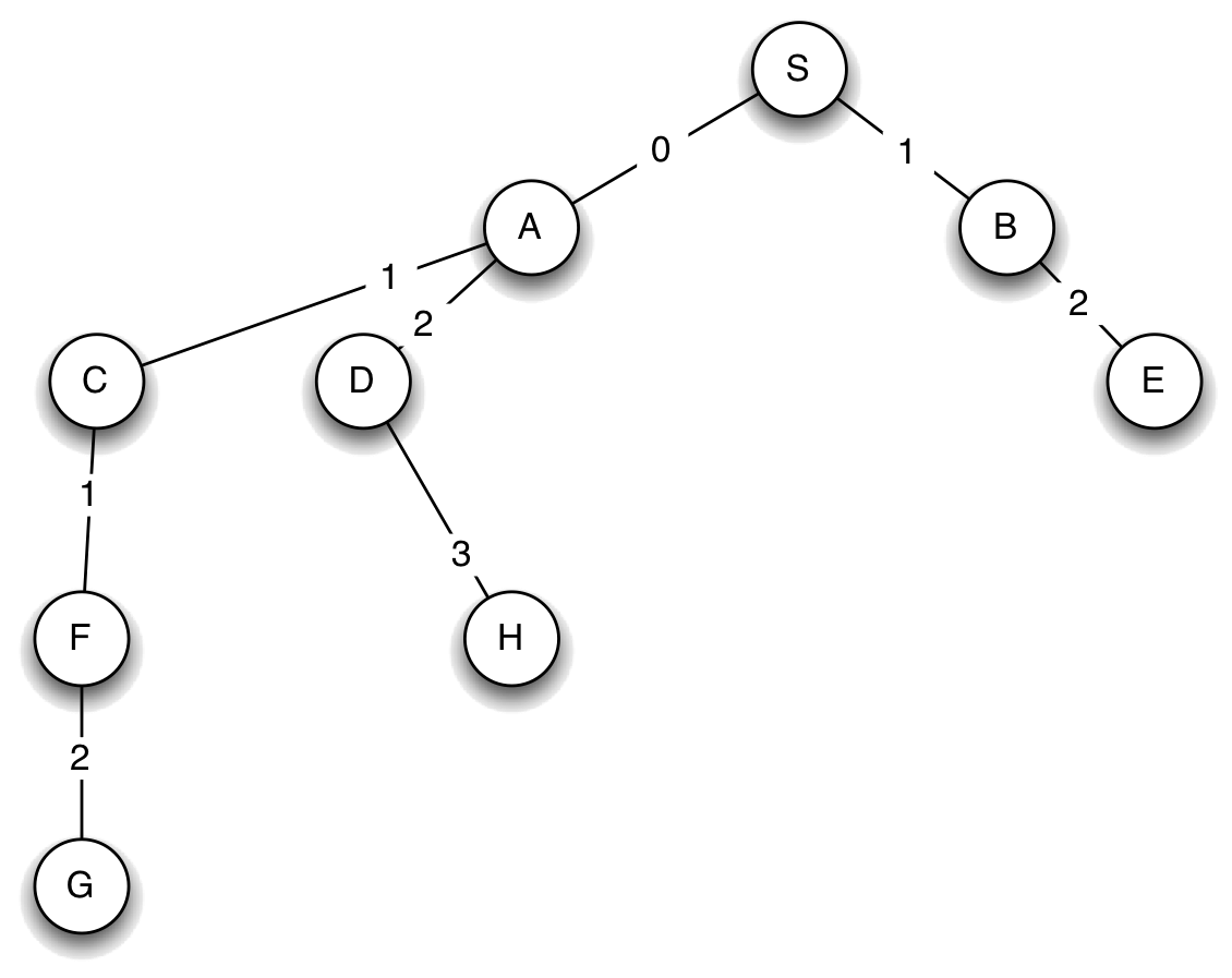
In bigger problems, this effect will be amplified to a large degree, and will make the difference between whether the algorithm can run in a reasonable amount of time, or not.
It is also worth noting that dynamic programming is guaranteed not to change the path returned by BFS; it simply helps us arrive at that solution more quickly.
We can make the same improvement to depth-first search; we just need to use a stack instead of a queue in the algorithm above. It still will not guarantee that the shortest path will be found, but will guarantee that we never visit more paths than the actual number of states.
6.4) Example: Numeric Search Domain
Many different kinds of problems can be formulated in terms of finding the shortest path through a space of states. Let's consider a search over a (potentially) less intuitive domain:
- The states are the integers.
- The initial state is some integer; let's say 1.
- Any state n has the following children: \{ 2n, n+1, n-1, n^2, -n\} .
- The goal test is lambda x: x == 10 .
So, the idea would be to find a short sequence of operations to move from 1 to 10.
Here it is, formalized in our Pythonic representation:
def successors(n):
    return [n*2, n+1, n-1, n**2, -n]

def goal_test(state):
    return state == 10

start_state = 1
First of all, this is a bad domain for applying depth-first search. Why? Because it will go off on a gigantic chain of doubling the starting state, and never find the goal. We can run breadth-first search, though. Without dynamic programming (but with pruning rules 1 and 2), here is what happens:
   expanding:  1
   expanding:  1 -(2*x)-> 2
   expanding:  1 -(x-1)-> 0
   expanding:  1 -(-x)-> -1
   expanding:  1 -(x*2)-> 2 -(x*2)-> 4
   expanding:  1 -(x*2)-> 2 -(x+1)-> 3
   expanding:  1 -(x*2)-> 2 -(-x)-> -2
   expanding:  1 -(x-1)-> 0 -(x-1)-> -1
   expanding:  1 -(-x)-> -1 -(x*2)-> -2
   expanding:  1 -(-x)-> -1 -(x+1)-> 0
   expanding:  1 -(x*2)-> 2 -(x*2)-> 4 -(x*2)-> 8
   expanding:  1 -(x*2)-> 2 -(x*2)-> 4 -(x+1)-> 5
33  states visited
Final path: [1, 2, 4, 5, 10]
We find a nice short path, but visit 33 states. Let's try it with DP:
   expanding:  1
   expanding:  1 -(x*2)-> 2
   expanding:  1 -(x-1)-> 0
   expanding:  1 -(-x)-> -1
   expanding:  1 -(x*2)-> 2 -(x*2)-> 4
   expanding:  1 -(x*2)-> 2 -(x+1)-> 3
   expanding:  1 -(x*2)-> 2 -(-x)-> -2
   expanding:  1 -(x*2)-> 2 -(x*2)-> 4 -(x*2)-> 8
   expanding:  1 -(x*2)-> 2 -(x*2)-> 4 -(x+1)-> 5
17  states visited
Final path: [1, 2, 4, 5, 10]
We find the same path, but visit noticeably fewer states. If we change the goal to 27, we find that we visit 564 states without DP and 119, with. If the goal is 1027, then we visit 12710 states without DP and 1150 with DP, which is getting to be a very big difference!
To experiment with depth-first search, we can make a version of the problem where the state space is limited to the integers in some range (without such a constraint, depth-first search would run forever):
def successors(n, max_value):
    return [min(max_value, max(i, -max_value)) for i in [n*2, n+1, n-1, n**2, -n]]

def goal_test(state):
    return state == 10

start_state = 1
Here's what happens if we give it a maximum value of 20:
   expanding:  1
   expanding:  1 -(-x)-> -1
   expanding:  1 -(-x)-> -1 -(x+1)-> 0
   expanding:  1 -(-x)-> -1 -(x*2)-> -2
   expanding:  1 -(-x)-> -1 -(x*2)-> -2 -(-x)-> 2
   expanding:  1 -(-x)-> -1 -(x*2)-> -2 -(-x)-> 2 -(x+1)-> 3
   expanding:  1 -(-x)-> -1 -(x*2)-> -2 -(-x)-> 2 -(x+1)-> 3 -(-x)-> -3
   expanding:  1 -(-x)-> -1 -(x*2)-> -2 -(-x)-> 2 -(x+1)-> 3 -(-x)-> -3 -(x**2)-> 9
20  states visited
[1, -1, -2, 2, 3, -3, 9, 10]
We generate a much longer path!
We can see from trying lots of different searches in this space that (a) the DP makes the search much more efficient and (b) that the difficulty of these search problems varies incredibly widely.
6.4.1) Search in lib601
lib601.search has implementats a single search procedure that can do either depth-first search or breadth-first search, both with dynamic programming.
from lib601.search import search

def successors(n, max_value):
    return [min(max_value, max(i, -max_value)) for i in [n*2, n+1, n-1, n**2, -n]]

def goal_test(state):
    return state == 10

start_state = 1

# Peforms breadth-first by default, keyword for depth-first
search(lambda n: successors(n, 20), start_state, goal_test, dfs=True)
6.5) Computational complexity
To finish up this segment, let's consider the computational complexity of these algorithms. As we've already seen, there can be a huge variation in the difficulty of a problem that depends on the exact structure of the graph, and is very hard to quantify in advance. It can sometimes be possible to analyze the average case running time of an algorithm, if you know some kind of distribution over the problems you're likely to encounter. We'll just stick with the traditional worst-case analysis, which tries to characterize the approximate running time of the worst possible input for the algorithm.
First, we need to establish a bit of notation. Let
- b be the branching factor of the graph; that is, the number of children a node can have. If we want to be truly worst-case in our analysis, this needs to be the maximum branching factor of the graph.
- d be the maximum depth of the graph; that is, the length of the longest path in the graph. In an infinite space, this could be infinite.
- l be the solution depth of the problem; that is, the length of the shortest path from the start state to the shallowest goal state.
- n be the state space size of the graph; that is the total number of states in the domain.
Depth-first search, in the worst case, will search the entire search tree. It has d levels, each of which has b times as many paths as the previous one. So, there are b^ d paths on the d^{th} level. The algorithm might have to visit all of the paths at all of the levels, which is about b^{d+1} states. But the amount of storage it needs for the agenda is only b \cdot d.
Breadth-first search, on the other hand, only needs to search as deep as the depth of the best solution. So, it might have to visit as many as b^{l+1} nodes. The amount of storage required for the agenda can be as bad as b^ l, too.
So, to be clear, consider the numeric search problem. The branching factor b = 5, in the worst case. So, if we have to find a sequence of 10 steps, breadth-first search could potentially require visiting as many as 5^{11} = 48828125 nodes!
This is all pretty grim. What happens when we consider the DP version of breadth-first search? We can promise that every state in the state space is visited at most once. So, it will visit at most n states. Sometimes n is much smaller than b^ l (for instance, in a road network). In other cases, it can be much larger (for instance, when you are solving an easy (short solution path) problem embedded in a very large space). Even so, the DP version of the search will visit fewer states, except in the very rare case in which there are never multiple paths to the same state (the graph is actually a tree). For example, in the numeric search problem, the shortest path from 1 to 91 is 9 steps long, but using DP it only requires visiting 1973 states, rather than 5^{10} = 9765625.
6.6) Uniform cost search
In many cases, some arcs in a graph will be more "preferable" than others. In a road network, we would really like to find the shortest path in miles (or in time to traverse), and different road segments have different lengths and times. To handle a problem like this, we need to extend our representation of search problems, and add a new algorithm to our repertoire.
Here is our original city map, now with distances associated with the roads between the cities.
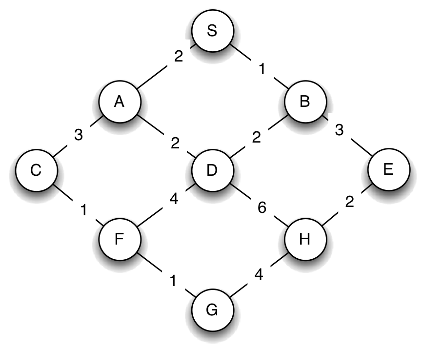
We can describe this map as a dictionary, this time associating a cost with each resulting state, as follows:
{'S' : (('A', 2), ('B', 1)),
 'A' : (('S', 2), ('C', 3), ('D', 2)),
 'B' : (('S', 1), ('D', 2), ('E', 3)),
 'C' : (('A', 3), ('F', 1)),
 'D' : (('A', 2), ('B', 2), ('F', 4), ('H', 6)),
 'E' : (('B', 3), ('H', 2)),
 'F' : (('C', 1), ('D', 4), ('G', 1)),
 'H' : (('D', 6), ('E', 2), ('G', 4)),
 'G' : (('F', 1), ('H', 4))}
When we studied breadth-first search, we argued that it found the shortest path, in the sense of having the fewest nodes, by seeing that it investigates all of the length 1 paths, then all of the length 2 paths, etc. This orderly enumeration of the paths guaranteed that when we first encountered a goal state, it would be via a shortest path. The idea behind uniform cost search is basically the same: we are going to investigate paths through the graph, in the order of the sum of the costs on their arcs. If we do this, we guarantee that the first time we extract a node with a given state from the agenda, it will be via a shortest path, and so the first time we extract a node with a goal state from the agenda, it will be an optimal solution to our problem.
6.6.1) Priority Queue
Just as we used a stack to manage the agenda for depth-first search and a queue to manage the agenda for bread-first search, we will need to introduce a new data structure, called a priority queue to manage the agenda for uniform-cost search. A priority queue is a data structure with the same basic operations as stacks and queues, with two differences:
- Items are pushed into a priority queue with a numeric score, called a cost.
- When it is time to pop an item, the item in the priority queue with the least cost is returned and removed from the priority queue.
There are many interesting ways to implement priority queues so that they are very computationally efficient, for example, Python has heapq. Here, we show a terrible, but very simple implementation, just to show what its behavior is supposed to be. Note that its data attribute consists of a list of (cost, item) pairs.
class PriorityQueue:
    def __init__(self):
        self.data = []
    def push(self, item, cost):
        self.data.append((cost, item))
    def pop(self):
        self.data.sort()
        return self.data.pop(0)[1]
    def is_empty(self):
        return len(self.data) == 0
6.6.2) Uniform-cost Search (UC)
Now, we're ready to study the uniform-cost search algorithm itself. We will start with a simple version that doesn't do any pruning or dynamic programming, and then add those features back in later.
First, we have to extend our definition of a SearchNode, to incorporate costs. So, when we create a new search node, we pass in an additional parameter cost, which represents the total cost of the path from the root of the tree to the node in question.
class SearchNode:
    def __init__(self, state, parent, cost=0):
        self.state = state
        self.parent = parent
        self.cost = cost

    def path(self):
        if self.parent == None:
            return [self.state]
        else:
            return self.parent.path() + [self.state]
Now, here is the search algorithm. It looks a lot like our standard search algorithm, but there are two important differences:
- The agenda is a priority queue.
- Instead of testing for a goal state when we put an element into the agenda, as we did in breadth-first search, we test for a goal state when we take an element out of the agenda. This is crucial, to ensure that we actually find the shortest path to a goal state.
def uniform_cost_search(successors, start_state, goal_test):
    if goal_test(start_state):
        return [start_state]
    start_node = SearchNode(start_state, None, 0)
    agenda = PriorityQueue()
    agenda.push(start_node, start_node.cost)
    while not agenda.is_empty():
        parent = agenda.pop()
        if goal_test(parent.state):
            return parent.path()
        for child_state, cost in successors(parent.state):
	    child = SearchNode(child_state, parent, parent.cost+cost)
            agenda.push(child, child.cost)
    return None
6.6.3) UC Example
Consider the following simple graph:
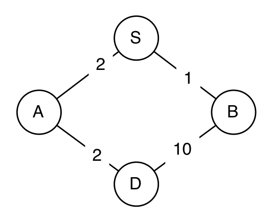
map = {'S' : (('A', 2), ('B', 1)),
       'A' : (('S', 2), ('D', 2)),
       'B' : (('S', 1), ('D', 10)),
       'D' : (('A', 2), ('B', 10))}

def successors(city):
    return map[city]

def goal_test(state):
    return state == 'D'

start_state = 'S'
Let's simulate the uniform-cost search algorithm:
- The agenda is initialized to contain the starting node. The agenda is shown as a list of cost, node pairs.
agenda: PQ([(0, S)])
- The least-cost node, S, is extracted and expanded, adding two new
nodes to the agenda. The notation S->A means that the path starts
in state S, and goes to state A.
0 : expanding: S agenda: PQ([(2, S->A), (1, S->B)]) - The least-cost node, S->B, is extracted, and expanded, adding
one new node to the agenda. Note, that, at this point, we have discovered a
path to the goal: S->B->D is a path to the goal, with cost 11.
But we cannot be sure that it is the shortest path to the goal, so we simply
put it into the agenda, and wait to see if it gets extracted before any other
path to a goal state.
1 : expanding: S->B agenda: PQ([(2, S->A), (11, S->B->D)]) - The least-cost node, S->A is extracted, and expanded, adding
one new node to the agenda. At this point, we have two different paths to the
goal in the agenda.
2 : expanding: S->A agenda: PQ([(11, S->B->D), (4, S->A->D)]) - Finally, the least-cost node, S->A->D is extracted. It is a
path to the goal, so it is returned as the solution.
5 states visited; Solution cost: 4
[(None, 'S'), (0, 'A'), (1, 'D')]
6.6.4) Dynamic programming
Now, we just need to add dynamic programming back in, but we have to do it slightly differently. We promise that, once we have expanded a node, that is, taken it out of the agenda, then we have found the shortest path to that state, and we need not consider any further paths that go through that state. So, instead of remembering which nodes we have visited (put onto the agenda) we will remember nodes we have expanded (gotten out of the agenda), and never visit or expand a node that has already been expanded. In the code below, the first test ensures that we don't expand a node that goes to a state that we have already found the shortest path to, and the second test ensures that we don't put any additional paths to such a state into the agenda.
def uniform_cost_search(successors, start_state, goal_test):
    if goal_test(start_state):
        return [start_state]
    start_node = SearchNode(start_state, None, 0)
    agenda = PriorityQueue()
    agenda.push(start_node, start_node.cost)
    expanded = set()
    while not agenda.is_empty():
        parent = agenda.pop()
        if parent.state not in expanded:
            expanded.add(parent.state)
            if goal_test(parent.state):
                return parent.path()
            for child_state, cost in successors(parent.state):
	        child = SearchNode(child_state, parent, parent.cost+cost)
                if child_state in expanded:
                    continue
                agenda.push(child, child.cost)
        return None
Here is the result of running this version of uniform cost search on our bigger city graph with distances:
agenda:  PQ([(0, S)])
    0 :   expanding:  S
agenda:  PQ([(2, S->A), (1, S->B)])
    1 :   expanding:  S->B
agenda:  PQ([(2, S->A), (3, S->B->D), (4, S->B->E)])
    2 :   expanding:  S->A
agenda:  PQ([(3, S->B->D), (4, S->B->E), (5, S->A->C), (4, S->A->D)])
    3 :   expanding:  S->B->D
agenda:  PQ([(4, S->B->E), (5, S->A->C), (4, S->A->D), (7, S->B->D->F), (9, S->B->D->H)])
    4 :   expanding:  S->B->E
agenda:  PQ([(5, S->A->C), (4, S->A->D), (7, S->B->D->F), (9, S->B->D->H), (6, S->B->E->H)])
agenda:  PQ([(5, S->A->C), (7, S->B->D->F), (9, S->B->D->H), (6, S->B->E->H)])
    5 :   expanding:  S->A->C
agenda:  PQ([(7, S->B->D->F), (9, S->B->D->H), (6, S->B->E->H), (6, S->A->C->F)])
    6 :   expanding:  S->B->E->H
agenda:  PQ([(7, S->B->D->F), (9, S->B->D->H), (6, S->A->C->F), (10, S->B->E->H->G)])
    6 :   expanding:  S->A->C->F
agenda:  PQ([(7, S->B->D->F), (9, S->B->D->H), (10, S->B->E->H->G), (7, S->A->C->F->G)])
agenda:  PQ([(9, S->B->D->H), (10, S->B->E->H->G), (7, S->A->C->F->G)])
13 states visited; Solution cost: 7
Final Path: ['S', 'A', 'C', 'F', 'G']
6.7) Search with heuristics
Ultimately, we'd like to be able to solve huge state-space search problems, such as those solved by a device that plans long routes through complex road networks using an initial position determined by a GPS receiver. We'll have to add something to uniform-cost search to solve such problems efficiently. Let's consider the city below, where the actual distances between the intersections are shown on the arcs:
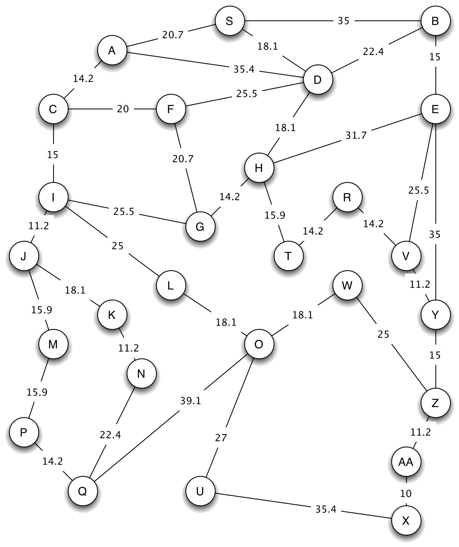
If we use uniform cost search to find a path from G to X, we expand states in the following order (the number at the beginning of each line is the length of the path from G to the state at the end of the path, as shown below:
    0 :   expanding:  G
    14.2 :   expanding:  G->H
    20.7 :   expanding:  G->F
    25.5 :   expanding:  G->I
    30.1 :   expanding:  G->H->T
    32.3 :   expanding:  G->H->D
    36.7 :   expanding:  G->I->J
    40.5 :   expanding:  G->I->C
    44.3 :   expanding:  G->H->T->R
    45.9 :   expanding:  G->H->E
    50.4 :   expanding:  G->H->D->S
    50.5 :   expanding:  G->I->L
    52.6 :   expanding:  G->I->J->M
    54.7 :   expanding:  G->H->D->B
    54.7 :   expanding:  G->I->C->A
    54.8 :   expanding:  G->I->J->K
    58.5 :   expanding:  G->H->T->R->V
    66.0 :   expanding:  G->I->J->K->N
    68.5 :   expanding:  G->I->J->M->P
    68.6 :   expanding:  G->I->L->O
    69.7 :   expanding:  G->H->T->R->V->Y
    82.7 :   expanding:  G->I->J->M->P->Q
    84.7 :   expanding:  G->H->T->R->V->Y->Z
    86.7 :   expanding:  G->I->L->O->W
    95.6 :   expanding:  G->I->L->O->U
    95.9 :   expanding:  G->H->T->R->V->Y->Z->AA
39 nodes visited; 27 states expanded; solution cost: 105.9
Final path: ['G', 'H', 'T', 'R', 'V', 'Y', 'Z', 'AA', 'X']
This search process works its way out, radially, from G, expanding nodes in contours of increasing path length. That means that, by the time the search expands node X, it has expanded every single node. This seems kind of silly: if you were looking for a good route from G to X, it's unlikely that states like S and B would ever come into consideration.
6.7.1) Heuristics
What is it about state B that makes it seem so irrelevant? Clearly, it's far away from where we want to go. We can incorporate this idea into our search algorithm using something called a heuristic function. A heuristic function takes a state as an argument and returns a numeric estimate of the total cost that it will take to reach the goal from there. We can modify our search algorithm to be biased toward states that are closer to the goal, in the sense that the heuristic function has a smaller value on them.
In a path-planning domain, such as our example, a reasonable heuristic is the actual Euclidean distance between the current state and the goal state; this makes sense because the states in this domain are actual locations on a map, and the Euclidean distance provides a lower bound on the length of any path between any two states.
6.7.2) A* Search (UC with Heuristic)
If we modify the uniform-cost search algorithm to take advantage of a heuristic function, we get an algorithm called A^* (pronounced "A-Star"). It is given below, with the differences highlighted in red. The only difference is that, when we insert a node into the priority queue, we do so with a cost that is new_node.cost + heuristic(new_state). That is, it is the sum of the actual cost of the path from the start state to the current state, and the estimated cost to go from the current state to the goal.
def a_star(successors, start_state, goal_test, heuristic=lambda x: 0):
    if goal_test(start_state):
        return [start_state]
    start_node = SearchNode(start_state, None, 0)
    agenda = PriorityQueue()
    agenda.push(start_node, heuristic(start_state))
    expanded = set()
    while not agenda.is_empty():
        parent = agenda.pop()
        if parent.state not in expanded:
            expanded.add(parent.state)
            if goal_test(parent.state):
                return parent.path()
            for child_state, cost in successors(parent.state):
                child = SearchNode(child_state, parent, parent.cost+cost)
                if child_state in expanded:
                    continue
                agenda.push(child, child.cost+heuristic(child_state))
        return None
6.7.3) A* Example
Now, we can try to search in the big map for a path from G to X, using, as our heuristic function, the distance between the state of interest and X. Here is a trace of what happens (with the numbers rounded to increase readability):
- We get the start node out of the agenda, and add its children. Note that
the costs are the actual path cost plus the heuristic estimate.
0 : expanding: G agenda: PQ([(107, G->I), (101, G->F), (79, G->H)]) - The least cost path is G->H, so we extract it, and add its
children.
14.2 : expanding: G->H agenda: PQ([(107, G->I), (101, G->F), (109, G->H->D), (116, G->H->E), (79, G->H->T)]) - Now, we can see the heuristic function really having an effect. The path
G->H->T has length 30.1, and the path G-1-F has length
20.7. But when we add in the heuristic cost estimates, the path to T
has a lower cost, because it seems to be going in the right direction. Thus, we
select G->H->T to expand next:
30.1 : expanding: G->H->T agenda: PQ([(107, G->I), (101, G->F), (109, G->H->D), (116, G->H->E), (100, G->H->T->R)]) - Now the path G->H->T->R looks best, so we expand it.
44.3 : expanding: G->H->T->R agenda: PQ([(107, G->I), (101, G->F), (109, G->H->D), (116, G->H->E), (103.5, G->H->T->R->V)]) - Here, something interesting happens. The node with the least estimated
cost is G->F. It's going in the wrong direction, but if we were to
be able to fly straight from F to X, then that would be a
good way to go. So, we expand it:
20.7 : expanding: G->F agenda: PQ([(107, G->I), (109, G->H->D), (116, G->H->E), (103.5, G->H->T->R->V), (123, G->F->D), (133, G->F->C)]) - Continuing now, basically straight to the goal, we have:
    58.5 :   expanding:  G->H->T->R->V
agenda:  PQ([(107, G->I), (109, G->H->D), (116, G->H->E), (123, G->F->D), (133, G->F->C), (154, G->H->T->R->V->E), (105, G->H->T->R->V->Y)])
    69.7 :   expanding:  G->H->T->R->V->Y
agenda:  PQ([(107, G->I), (109, G->H->D), (116, G->H->E), (123, G->F->D), (133, G->F->C), (154, G->H->T->R->V->E), (175, G->H->T->R->V->Y->E), (105, G->H->T->R->V->Y->Z)])
    84.7 :   expanding:  G->H->T->R->V->Y->Z
agenda:  PQ([(107, G->I), (109, G->H->D), (116, G->H->E), (123, G->F->D), (133, G->F->C), (154, G->H->T->R->V->E), (175, G->H->T->R->V->Y->E), (151, G->H->T->R->V->Y->Z->W), (106, G->H->T->R->V->Y->Z->AA)])
    95.9 :   expanding:  G->H->T->R->V->Y->Z->AA
agenda:  PQ([(107, G->I), (109, G->H->D), (116, G->H->E), (123, G->F->D), (133, G->F->C), (154, G->H->T->R->V->E), (175, G->H->T->R->V->Y->E), (151, G->H->T->R->V->Y->Z->W), (106, G->H->T->R->V->Y->Z->AA->X)])
18 nodes visited; 10 states expanded; solution cost: 105.9
[(None, 'G'), (2, 'H'), (2, 'T'), (1, 'R'), (1, 'V'), (2, 'Y'), (2, 'Z'), (2, 'AA'), (1, 'X')]
Using A* has roughly halved the number of nodes visited and expanded. In some problems it can result in an enormous savings, but, as we'll see in the next section, it depends on the heuristic we use.
6.7.4) Good and Bad Heuristics
In order to think about what makes a heuristic good or bad, let's imagine what the perfect heuristic would be. If we were to magically know the distance, via the shortest path in the graph, from each node to the goal, then we could use that as a heuristic. It would lead us directly from start to goal, without expanding any extra nodes. But, of course, that's silly, because it would be at least as hard to compute the heuristic function as it would be to solve the original search problem.
So, we would like our heuristic function to give an estimate that is as close as possible to the true shortest-path-length from the state to the goal, but also to be relatively efficient to compute.
An important additional question is: if we use a heuristic function, are we still guaranteed to find the shortest path through our state space? The answer is: yes, under certain conditions.
Without dynamic programming, A^* is guaranteed to return an optimal (least-cost) path if the heuristic function is admissible. A heuristic function is admissible if it is guaranteed not to overestimate the actual cost of the optimal path to the goal. To see why this is important, consider a state s from which the goal can actually be reached in 10 steps, but for which the heuristic function gives a value of 100. Any path to that state will be put into the agenda with a total cost of 90 more than the true cost. That means that if a path is found that is as much as 89 units more expensive that the optimal path, it will be accepted and returned as a result of the search.
With dynamic programming, A^* is only guaranteed to return an optimal path if its heuristic is consistent, which is a slightly stronger condition than admissibility. A heuristic function h is consistent if the heuristic evaluated at the goal state is 0, and, for every state s and for every successor s' of s, the estimated cost of reaching the goal h(n) is no greater than the step cost of getting to s' plus the estimated cost h(s'):
Note that, while all consistent heuristics are admissible, not all admissible heuristics are consistent! That said, most sensible admissible heuristics are also consistent (it takes some effort to come up with a heuristic that is admissible but not consistent).
To see why this condition is necessary, consider searching from state (0, 0) to state (100, 0) in a rectangular grid. Obviously, the shortest path between these two states is a straight line. Now consider searching with the following (admissible) heuristic):
With this heuristic, the search will return the optimal path if we are not using dynamic programming (since it is admissible), but if we are using dynamic programming, the search will go around state (1,0) and return a sub-optimal path!
It is important to see that if our heuristic function always returns value 0, it is both admissible and consistent. And, in fact, with that heuristic, the A^* algorithm reduces to uniform cost search.
In the example of navigating through a city, we used the Euclidean distance between cities, which, if distance is our cost, is clearly admissible; there's no shorter path between any two points.
It is worth noting that, if we do not care about getting the shortest path to the goal, but rather about getting any path to the goal, then it is fine to use a non-admissible heuristic. When implemented properly, this can intensify the effect the heuristic will have on "nudging" our search toward the goal. For example, using the square of the Euclidean distance would have this effect, but we would lose the guarantee of UC returning the shortest path to the goal.
Would the so-called 'Manhattan distance', which is the sum of the absolute differences of the x and y coordinates be an admissible heuristic in the city navigation problem, in general? Would it be admissible in a city whose roads make up a perfect grid with no diagonals?
If we were trying to minimize travel time on a road network (and so the estimated time to travel each road segment was the cost), what would be an appropriate heuristic function?
6.7.5) Heuristic Search in lib601
lib601.search has an implementation of uniform_cost_search. This procedure has an optional heuristic keyword argument that defaults to a heuristic that always returns 0. This procedure can be used for both uniform cost search and for A* search.
from lib601.search import uniform_cost_search

map = {'S' : (('A', 2), ('B', 1)),
       'A' : (('S', 2), ('D', 2)),
       'B' : (('S', 1), ('D', 10)),
       'D' : (('A', 2), ('B', 10))}

def successors(city):
    return map[city]

def goal_test(state):
    return state == 'D'

start_state = 'S'

uniform_cost_search(successors, start_state, goal_test, heuristic=lambda s:0)
Footnotes
1Although in many cases we have a particular goal state, in other cases, we may have the goal of going to any gas station, which can be satisfied by many different intersections.
2We will discuss our Pythonic representation for state-space search more compltetly later in the chapter.
3It is sufficient to take only the successors, start_state and the goal_test function as input, as these three together completely specify our search problem. Note that the set of all possible states is not explicitly specified.
4Python implements a set data type that supports checking membership (via in) efficiently (in time independent of the number of elements in the set). You could also use a list, but the performance would be noticeably worse in any nontrivial search domain in works in linear time for lists, but constant time for sets.