5) Probability 2

Table of Contents

• 5) Probability 2
• 5.1) Introduction
• 5.2) Python operations on distributions
• 5.2.1) Constructing a joint distribution
• 5.2.2) Conditioning
• 5.2.3) Bayesian Evidence
• 5.2.4) Total Probability
• 5.3) Modeling with distributions
• 5.4) Primitives
• 5.4.1) Delta
• 5.4.2) Uniform
• 5.4.3) Square
• 5.4.4) Triangle
• 5.5) Mixture distribution
• 5.6) Stochastic state machines
• 5.7) Markov chains
• 5.8) Python representation
• 5.8.1) Probability of a sequence
• 5.8.2) Distribution at time t
• 5.8.3) Limiting distribution
• 5.9) Hidden Markov models
• 5.10) Copy machine example
• 5.11) State estimation
• 5.12) Our first copy
• 5.13) Our second copy
• 5.14) General state estimation

5.1) Introduction

In the last chapter, we discussed the mathematics of Probability Theory as a means of making precise statements about uncertain situations, and to characterize our uncertainty about these situations.

5.2) Python operations on distributions

We can implement the operations described in the previous chapter as operations on DDist instances.

5.2.1) Constructing a joint distribution

We start by defining a procedure that takes a distribution \Pr (A), named PA, and a conditional distribution \Pr (B \mid A), named prob_b_given_a, and returns a joint distribution \Pr (A, B), represented as a Python dist.DDist instance. It must be the case that the domain of A in PA is the same as in prob_b_given_a. It creates a new instance of dist.DDist with entries (a, b) for all a with support in PA and b with support in PB. The Python expression PA.prob(a) corresponds to \Pr (A = a) ; prob_b_given_a is a conditional probability distribution, so prob_b_given_a(a) is the distribution \Pr (B \mid A = a) on B , and prob_b_given_a(a).prob(b) is \Pr (B = b \mid A = a).

So, for example, we can re-do our joint distribution on A and B as:

PA = dist.DDist({'a1' : 0.9, 'a2' : 0.1})
def prob_b_given_a(a):
    if a == 'a1':
        return dist.DDist({'b1' : 0.7, 'b2' : 0.3})
    else:
        return dist.DDist({'b1' : 0.2, 'b2' : 0.8})
>>> PAB = dist.make_joint_distribution(PA, prob_b_given_a)
>>> PAB
DDist((a1, b2): 0.270000, (a1, b1): 0.630000, (a2, b2): 0.080000, (a2, b1): 0.020000)

We have constructed a new joint distribution. We leave the implementation as an exercise.

5.2.2) Conditioning

We can also add a condition_on_var method to DDist which, like marginalize_out, should only be applied to joint distributions. It takes as input an index of the value to be conditioned on, and a value for that variable, and returns a DDist on the remaining variables. It operates in three steps:

• Collect all of the value-tuples in the joint distribution that have the specified value at the specified index. This is the new universe of values, over which we will construct a distribution.

• Compute the sum of the probabilities of those elements.

• Create a new distribution by removing the elements at the specified index (they are redundant at this point, since they are all equal) and dividing the probability values by the sum of the probability mass in this set. The result is guaranteed to be a distribution in the sense that the probability values properly sum to 1.

Now, we can compute, for example, the distribution on A, given that B = b_1 :

>>> PAB.condition_on_var(1, 'b1')
DDist(a1: 0.969231, a2: 0.030769)

Note that this is not a conditional distribution, because it is not a function from values of B to distributions on A . At this point, it is simply a distribution on A .

So, this method takes an index (of the variable we are conditioning on) and returns a conditional probability distribution of the other variables in the joint distribution, given the variable at the specified index.

Answer:

def cond_dist(self, index):
return lambda val: self.condition_on_var(index, val)

5.2.3) Bayesian Evidence

The operation of updating a distribution on a random variable A , given evidence in the form of the value b of a random variable B , can be implemented as a procedure that takes as arguments the prior distribution \Pr (A) , named PA, a conditional distribution \Pr (B \mid A) , named prob_b_given_a, and the actual evidence b , named b. It starts by constructing the joint distribution \Pr (A, B) with make_joint_distribution. Then, remembering that the order of the variables in the joint distribution is (A, B), it conditions on the variable with index 1 (that is, B ) having value b, and returns the resulting distribution over A .

So, for example, given a prior distribution on the prevalence of disease in the population

pDis = dist.DDist({True: 0.001, False: 0.999})

and the conditional distribution of test results given disease:

def prob_test_given_dis(disease):
    if disease:
        return dist.DDist({True: 0.99, False: 0.01})
    else:
        return dist.DDist({True: 0.001, False: 0.999})

we can determine the probability that someone has the disease if the test is positive:

>>> dist.bayes_rule(pDis, prob_test_given_dis, True)
DDist(False: 0.502262, True: 0.497738)

5.2.4) Total Probability

Finally, we can implement the law of total probability straightforwardly in Python. Given a distribution \Pr (A) , called PA, and \Pr (B \mid A) , called prob_b_given_a, we compute \Pr (B) . We do this by constructing the joint distribution and then marginalizing out A (which is the variable with index 0).

To compute the probability distribution of test results in the example above, we can do:

>>> dist.total_probability(pDis, prob_test_given_dis)
DDist(False: 0.998011, True: 0.001989)

5.3) Modeling with distributions

When we have a small number of discrete states, it is relatively easy to specify probability distributions. But, as domains become more complex, we will need to develop another PCAP system, just for constructing distributions. In this section, we'll describe a collection of relatively standard primitive distributions, and a method, called a mixture distribution for combining them, and show how they can be implemented in Python.

5.4) Primitives

5.4.1) Delta

Sometimes we'd like to construct a distribution with all of the probability mass on a single element. Here's a handy way to create delta distributions, with a probability spike on a single element:

def delta_dist(v):
    return DDist({v:1.0})

5.4.2) Uniform

Another common distribution is the uniform distribution. On a discrete set of size n , it assigns probability 1/ n to each of the elements:

def uniform_dist(elts):
    p = 1.0 / len(elts)
    return DDist(dict([(e, p) for e in elts]))

5.4.3) Square

There are some distributions that are particularly valuable in numeric spaces. Since we are only dealing with discrete distributions, we will consider distributions on the integers.

One useful distribution on the integers is a square distribution. It is defined by parameters lo and hi, and assigns probability

to all integers from \textit{lo} to \textit{hi} - 1 . Here is a square distribution (from 60 to 80):

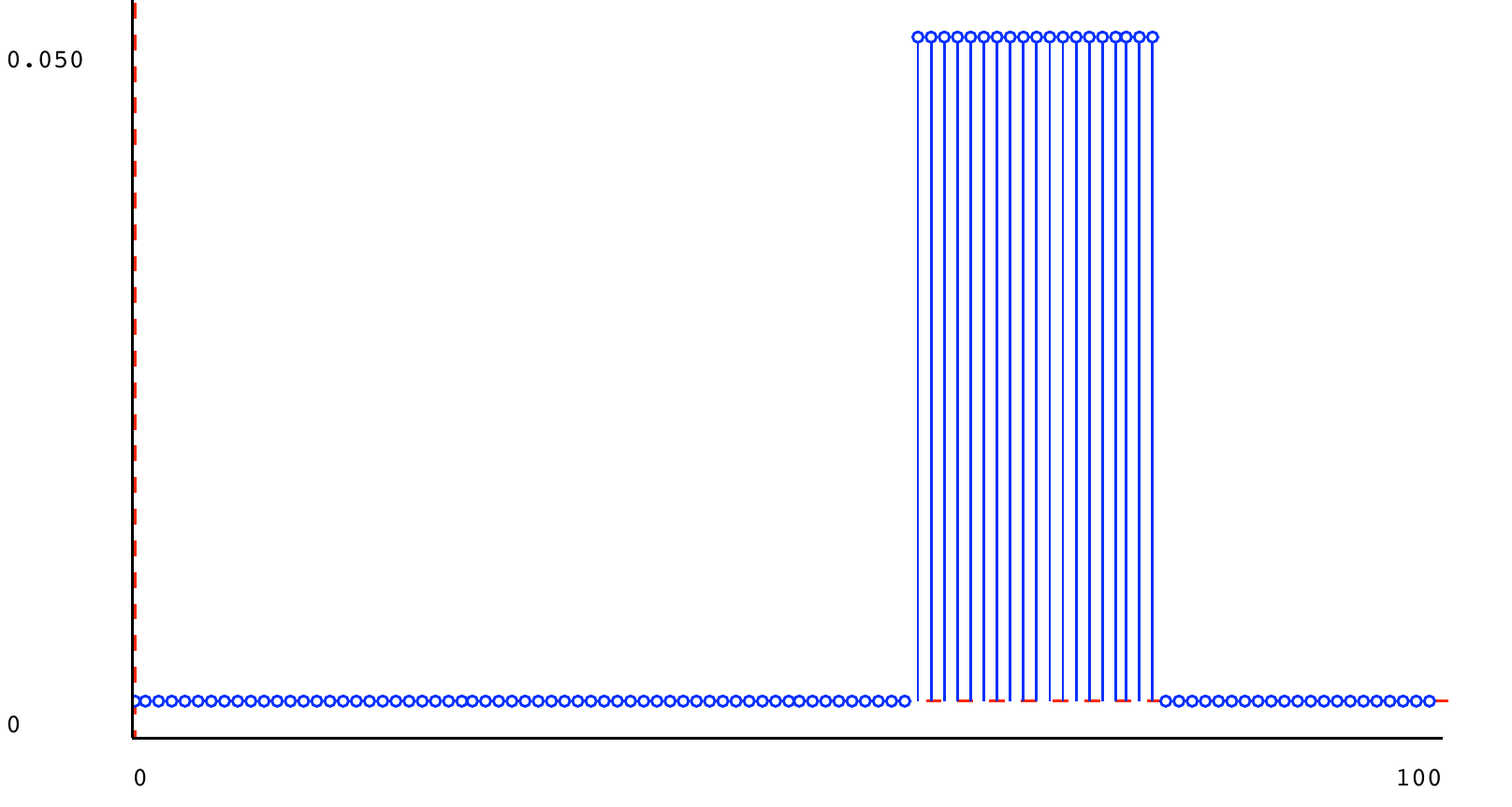
Because it is non-zero on 20 values, those values have probability 0.05 .

5.4.4) Triangle

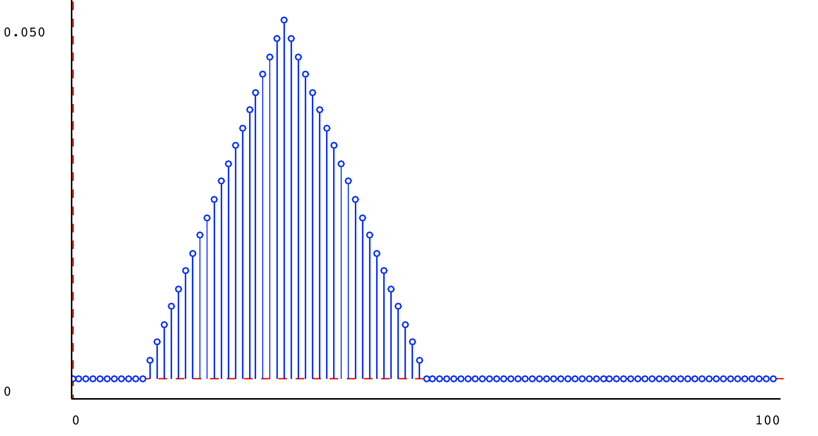
Another useful distribution is a triangle distribution. It is defined by parameters peak and halfWidth. It defines a shape that has its maximum value at index peak, and has linearly decreasing values at each of \textit{halfWidth} - 1 points on either side of the peak. The values at the indices are scaled so that they sum to 1. Here is a triangular distribution with peak 30 and half-width 20.

5.5) Mixture distribution

We can combine distributions by mixing them. To create a mixture distribution, we specify two distributions, d_1 and d_2 and a mixing parameter p , with 0 \leq p \leq 1 . The intuition is that, to draw an element from a mixture distribution, first we first flip a coin that comes up heads with probability p . If it is heads, then we make a random draw from d_1 and return that; otherwise we make a random draw from d_2 and return it. Another way to see it is that, if we think of a random variable D_1 having distribution d_1 and another random variable D_2 having distribution d_2 , then

that is, the probability of an element x under the mixture distribution is p times its probability under distribution d_1 plus 1-p times its probability under distribution d_2 .

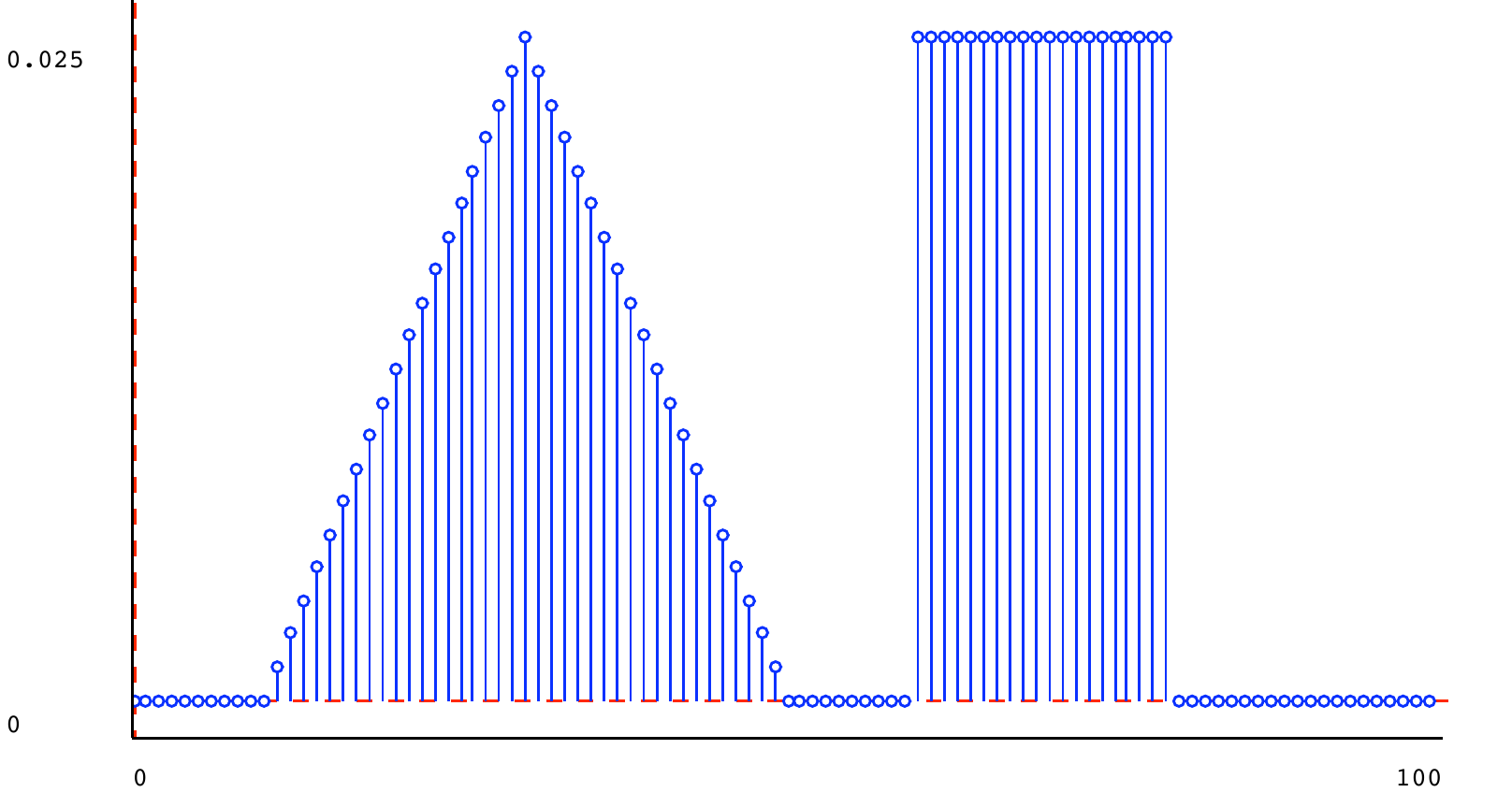
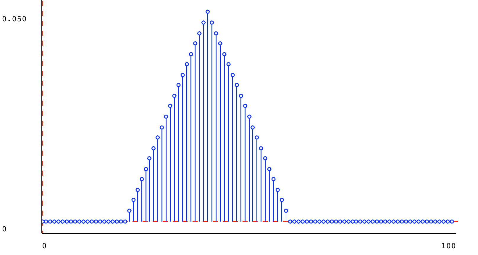
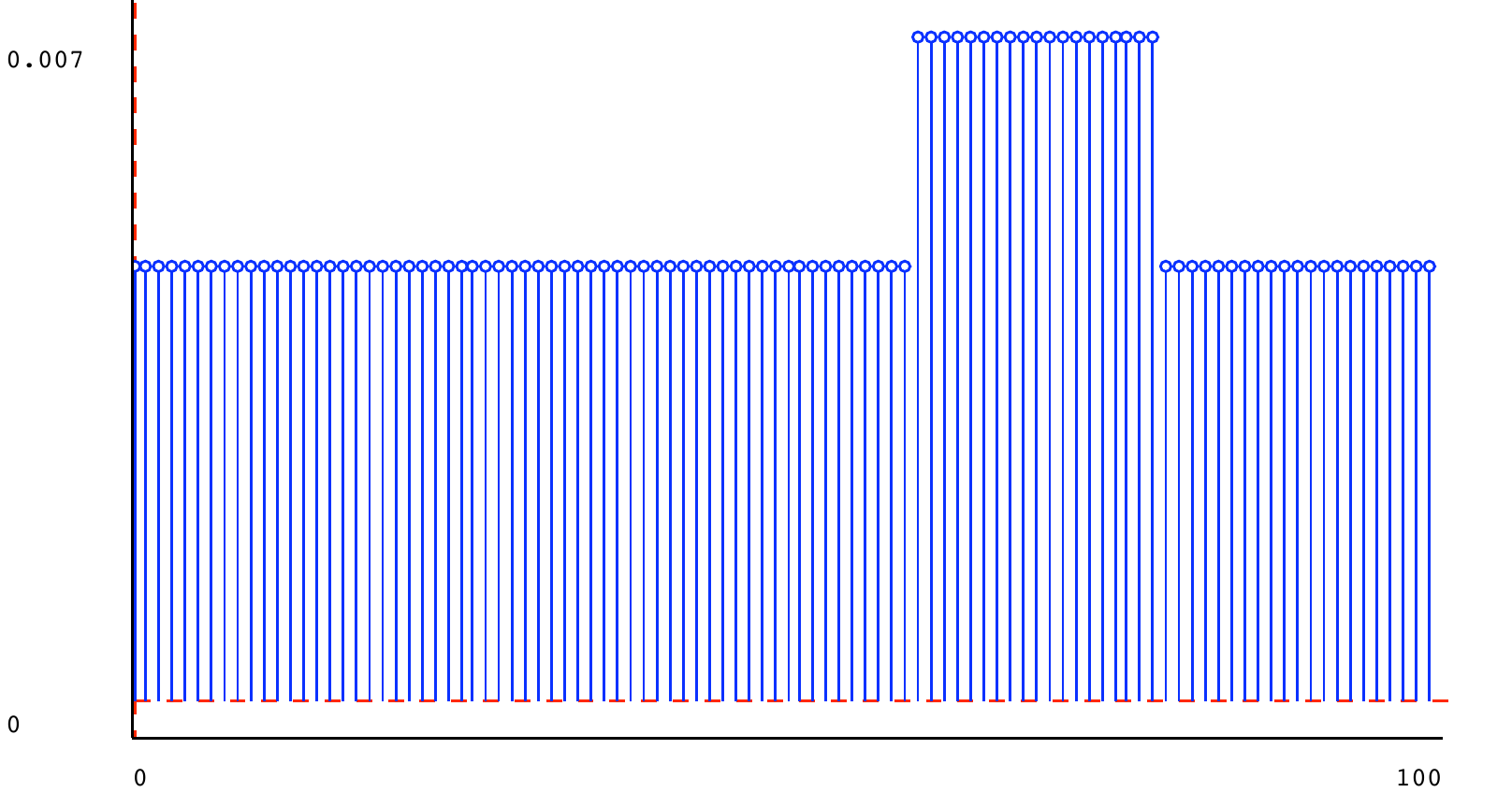
We can make a mixture of the square and triangle distributions shown above, with mixture parameter 0.5:

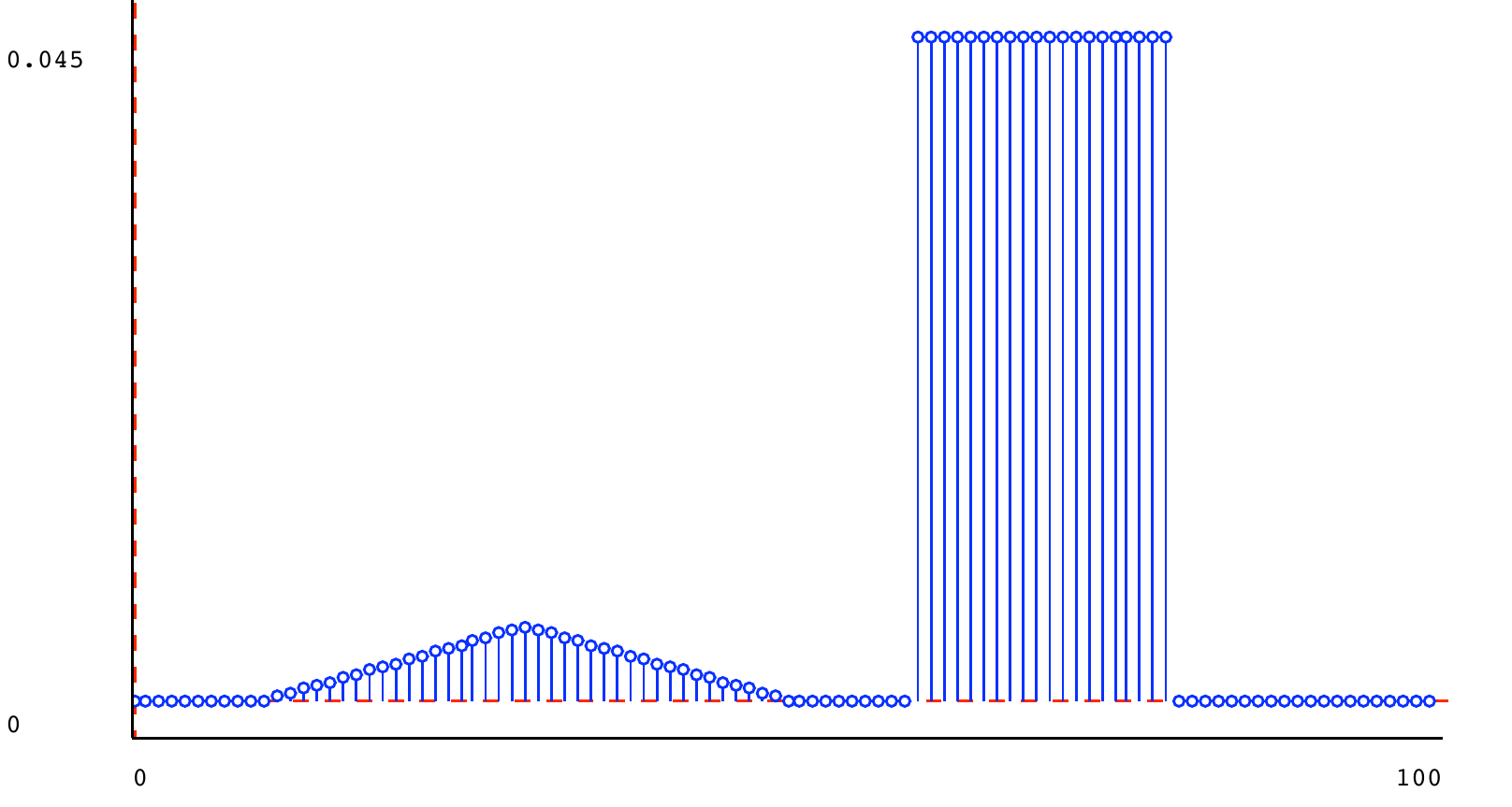
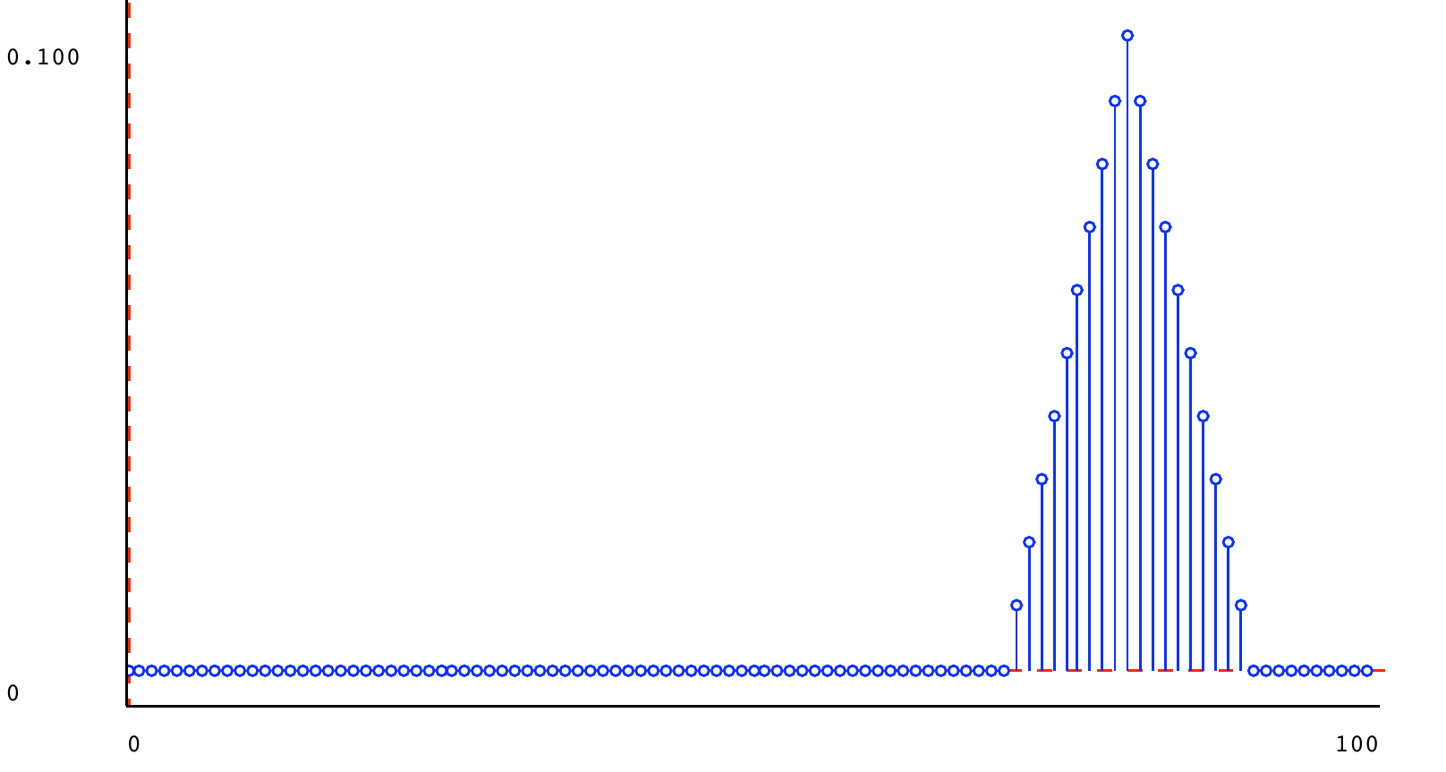
Here it is, with mixture parameter 0.9, where the square is d_1 and the triangle is d_2 :

To implement a mixture distributions, we have two choices. One would be to go through the supports of both component distributions and create a new explicit DDist. Below, we have taken the 'lazy' approach, similar to the way we handled signal composition. We define a new class that stores the two component distributions and the mixture parameter, and computes the appropriate probabilities as necessary.

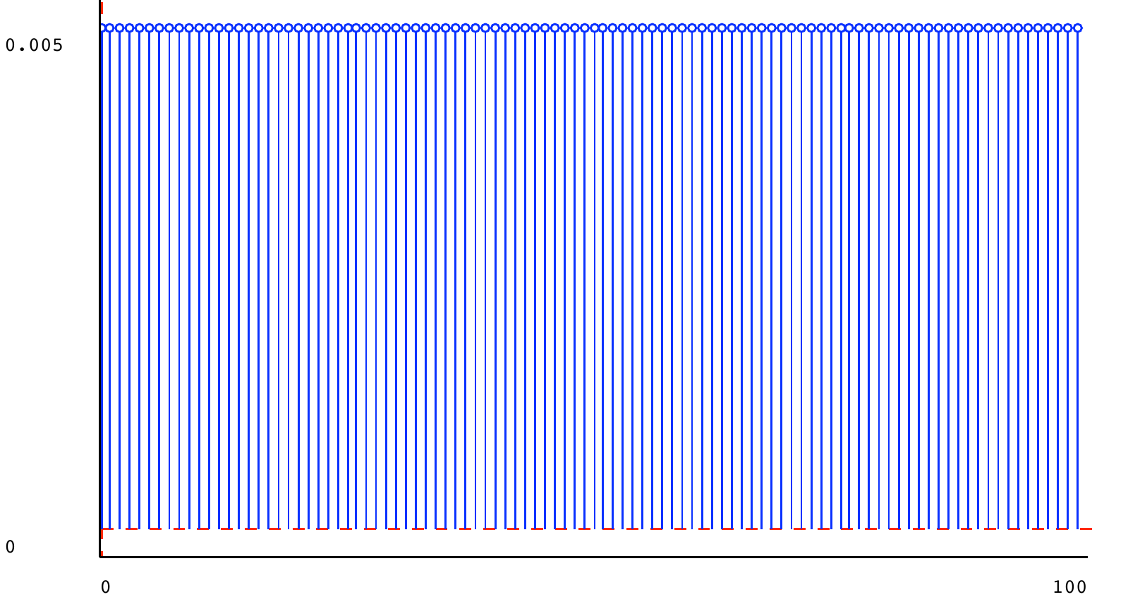
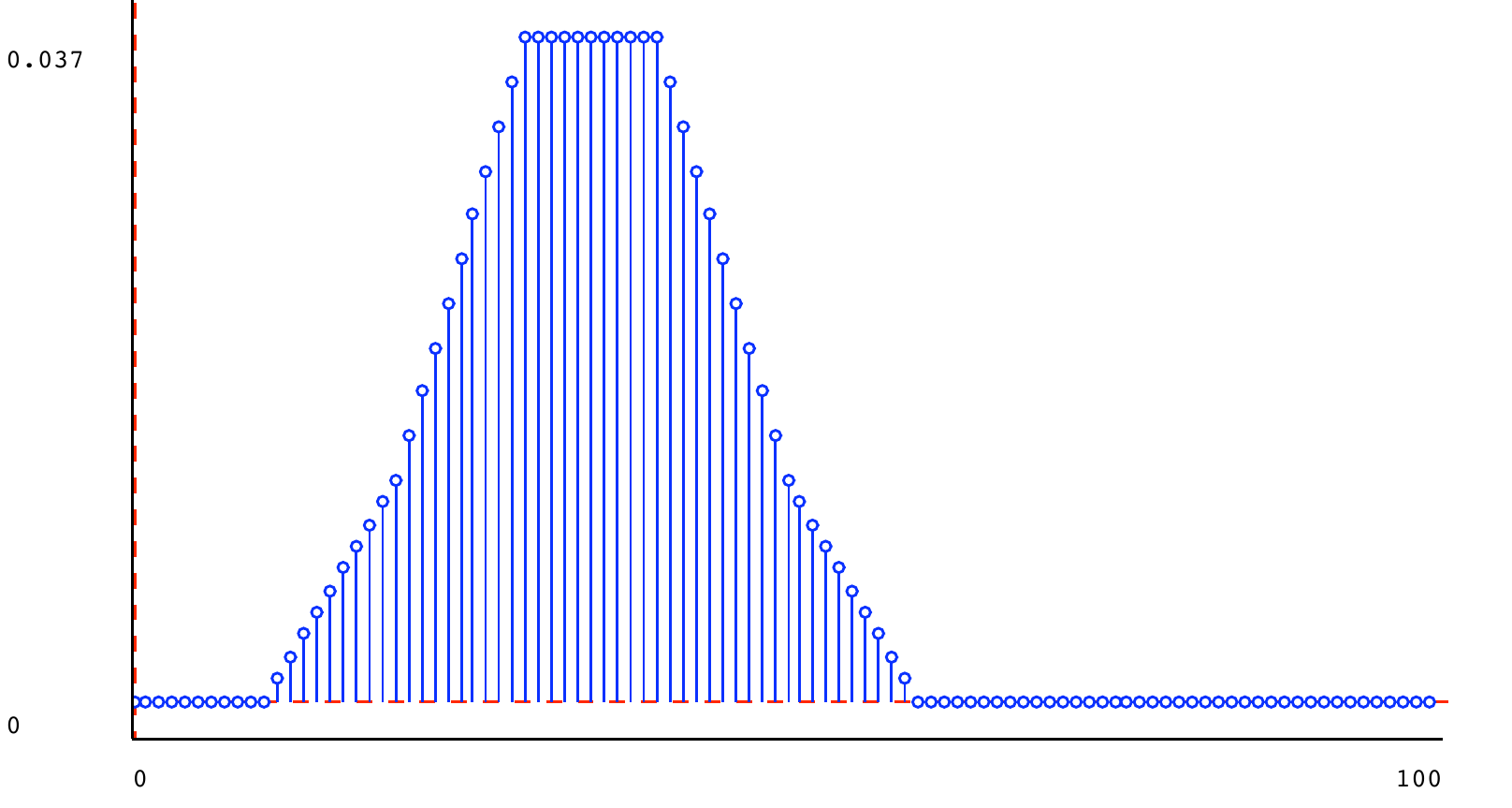
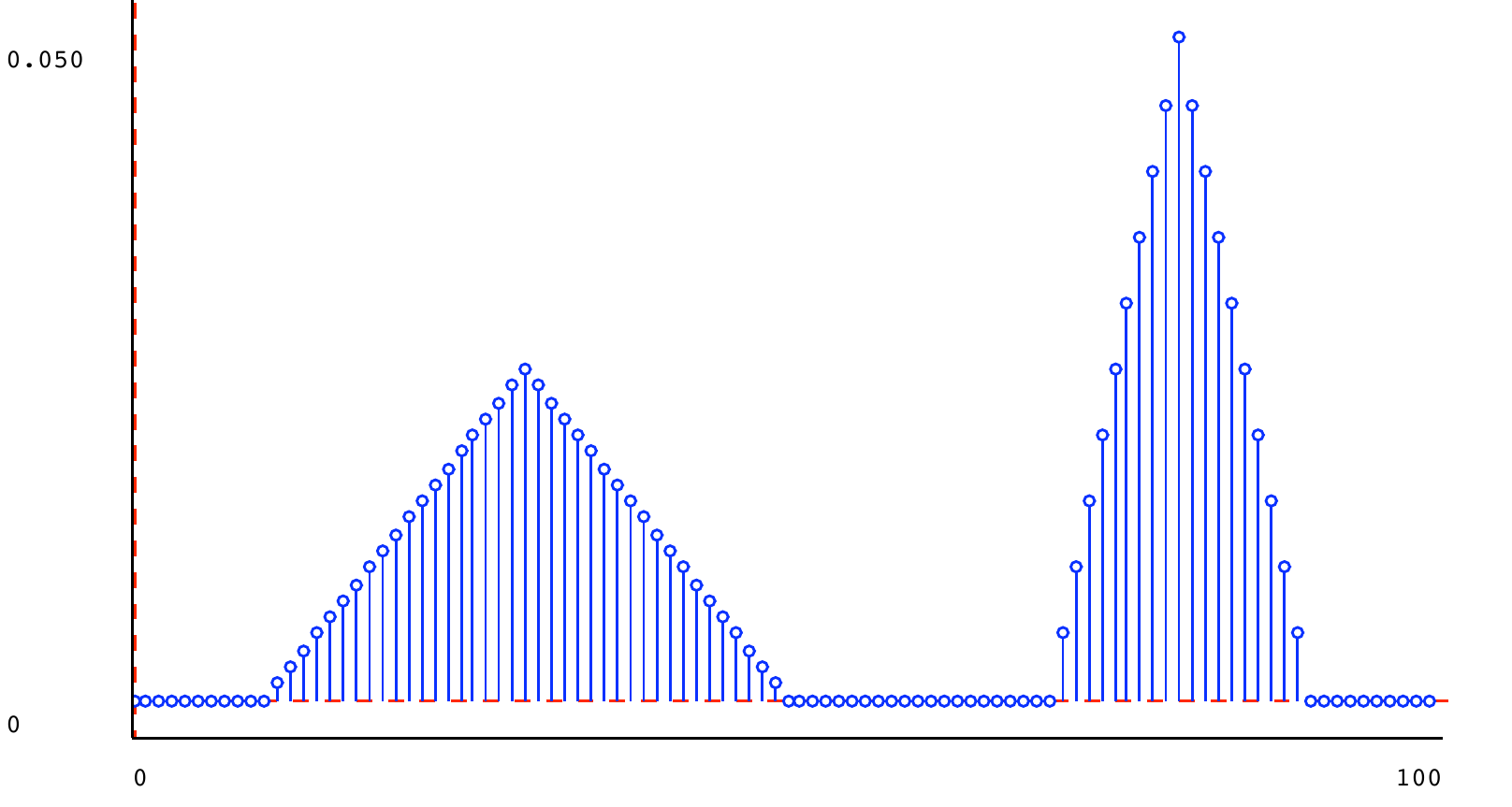
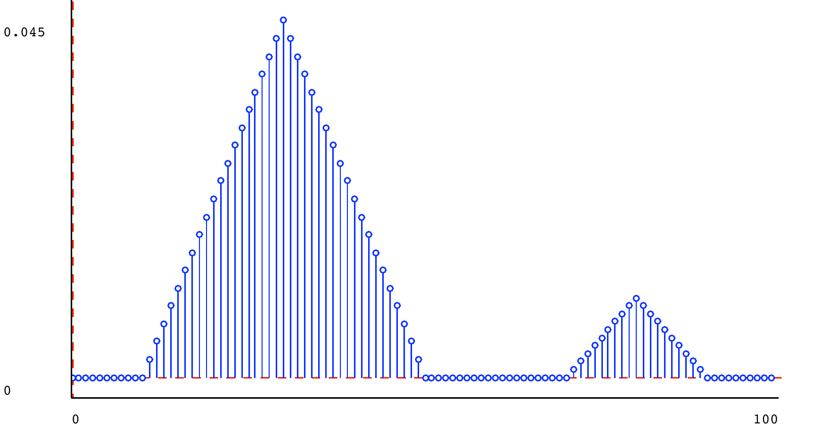
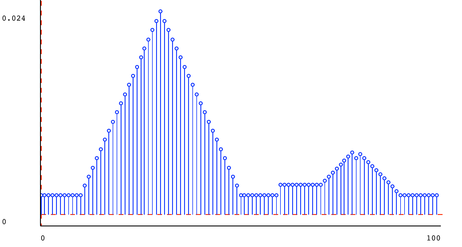
Here are some example mixture distributions, created in Python and plotted below.

t1 = dist.triangle_dist(30, 20)
t2 = dist.triangle_dist(40, 20)
t3 = dist.triangle_dist(80, 10)
s1 = dist.square_dist(0, 100)
s2 = dist.square_dist(60, 80)
m1 = dist.mixture(t1, t2, 0.5)
m2 = dist.mixture(s1, s2, 0.95)
m3 = dist.mixture(t1, t3, 0.5)
m4 = dist.mixture(t1, t3, 0.9)
m5 = dist.mixture(m2, m4, 0.5)

5.6) Stochastic state machines

As we saw earlier, a state machine is a model of some process that changes over time. LTI systems are one kind of state machine, in which the state is some vector of previous inputs and outputs, and the output at each step is a linear function of the input and the values in the state. LTI systems are infinite state: the possible internal states are vectors of real numbers, and it is generally not the case that they will ever revisit a state. We also looked at finite state machines, in which we could characterize the transition function and output function using simple tables.

In this section, we will consider state machines that have a finite number of possible states, but are more interesting in that they don't behave deterministically. Instead of the next state being determined from the previous state and input by looking them up in a table, the next state will be drawn from a probability distribution that depends on the previous state and input. The output generated by the machine will be drawn from a probaiblity distriution, as well. The general case is pretty complicated, so we will work up to it in stages.

5.7) Markov chains

We'll start by thinking just about state transitions, and not worry about inputs or outputs (if you want to, you can think of the case where the output is equal to the state of the machine, and where the next state depends only on the previous state, and not on the input). A finite state machine whose next state depends probabilistically on the previous state is called a Markov chain.

Mathematically, we can specify a Markov chain with three components:

• States {\cal S}

• Initial state distribution \Pr (S_0)

• Transition distribution \Pr (S_{t+1} \mid S_ t) . Because the process is time-invariant, this is the same for all t .

There is a finite set of possible states {\cal S} . We will use random variables S_ t to stand for the state of the system at time t ; these random variables can have values in {\cal S} .

The initial state, S_0 , is a random variable: we don't even (necessarily) know where we will start! We specify a distribution over the starting state with \Pr (S_0) .

Then, to specify how the state changes over time, we have to specify a conditional probability distribution \Pr (S_{t+1} \mid S_ t) . Given a state at some time step t , called S_ t , it specifies a distribution over the state at the next time step, S_{t+1} . Markov chains are time invariant: that is, although the state may change over time, the probability distribution governing these changes stays constant.

Furthermore their state transitions are Markov: that is, the state at time t+1 is conditionally independent of all previous states, given the state at time t . Another way to say that is: the state at time t is all you need to make the best possible prediction of the state at time t+1 ; knowing any or all of the states before that won't help you make a better prediction.

As a very simple example, let's consider a copy machine: we'll model it in terms of two possible internal states: good and bad. Here is a specification of it.

• States: \{ \textit{good}, \textit{bad}\}

• Initial state distribution:

  \Pr (S_0) = \{ \textit{good} : 0.9, \textit{bad}: 0.1\}

• Transition distribution:

  \Pr (S_{t+1} \mid S_ t) = \begin{cases} \{ \textit{good} : 0.7, \textit{bad}: 0.3\} & if S_ t = \textit{good} \\ \{ \textit{good} : 0.1, \textit{bad}: 0.9\} & if S_ t = \textit{bad} \\ \end{cases}

It will initially start out in the state good (meaning that it is basically functioning well) with reasonably high probability (0.9 ). But, its state may change on every time step. For concreteness, let's assume that a "time step" for this process occurs every time we use the machine to make a copy.

Remember that the transition distribution is a conditional probability distribution, and that a conditional distribution is actually a function from values of the variable that is being conditioned on (in this case, S_ t ) to distributions over the variable on the left (in this case, S_{t+1} ). This particular transition distribution says that, if the machine was in a good state at time t , then with probability 0.7 it will stay good, and with probability 0.3 , it will transition to the bad state at time t+1 . (That's a pretty terrible machine!). If it is in a bad state at time t , then with probability 0.1 it miraculously becomes good, and with probability 0.9 it stays bad at time t+1 .

5.8) Python representation

We can represent these basic distributions in Python using the DDist class that we have already developed. First, we have the initial state distribution, which is quite straightforward:

initial_state_distribution = dist.DDist({'good': 0.9, 'bad': 0.1})

The transition distribution is a conditional probability distribution:

def transition_distribution(oldState):
    if oldState == 'good':
        return dist.DDist({'good' : 0.7, 'bad' : 0.3})
    else:
        return dist.DDist({'good' : 0.1, 'bad' : 0.9})

Finally, we can define a new class, called MarkovChain.

class MarkovChain:
    def __init__(self, start_distribution, transition_distribution)
        self.start_distribution = start_distribution
        self.transition_distribution = transition_distribution

Now, we can define our copy machine:

copyMachine = MarkovChain(initial_state_distribution, transition_distribution)

Questions about Markov chains

There are a number of interesting questions we can ask about a Markov chain. Let's explore how to answer them with the probability theory we know.

5.8.1) Probability of a sequence

One might be interested in the question, how likely is it that the system will go through some particular sequence of states s_0, s_1, \ldots , s_ T . That is, we're interested in

We can use the operation of conditioning to rewrite this as:

That's still pretty ugly. But, because of the Markov property, we can simplify it to:

which, if we're feeling fancy, we can finally write as:

We can use the definition above to get:

All those probabilities are given in the initial distribution and the transition distribution. So, we have

5.8.2) Distribution at time t

Rather than asking about a particular trajectory through the state space, we might want to know, more generally, how likely the machine is to be in some state at a particular time (without caring so much about how it got there). That is, we could be interested in:

This problem seems like it might be tricky, but we can apply some tools from the previous section. Mostly we will be interested in the law of total probability. We can write

That says that, in order to think about the probability that the state of the system at time T is s_ T , we have to marginalize over all possible sequences states that end in s_ T . Yikes!! If T is very big, then that's a lot of sequences.

Luckily, the Markov property comes to the rescue. To determine the distribution over states at time T , it is sufficient to know the distribution at the previous time step. We can exploit that property to develop a more efficient algorithm.

Let's start by thinking about the state distribution at time 0. That's easy. It's just the starting distribution \Pr (S_0) , which we know.

Now, how do we get the distribution over the state at time 1? We can make the joint on S_0 and S_1 and then marginalize out S_0 .

We even have a compact way of thinking of this as the law of total probability. This should now suggest a way of proceeding in general:

This is a kind of dynamic programming algorithm: it makes use of intermediate results (the occupation disributions at earlier time steps) to efficiently calculate a final result, without enumerating all possible state sequences.

5.8.3) Limiting distribution

For some distributions, if we let t approach \infty , the occupation distribution at time t converges to some fixed distribution. We can call this the stationary or limiting distribution. The exact condition under which such a distribution exists is a little bit complicated, but we can definitely guarantee that it exists if \Pr (S_{t+1} = s_ i \mid S_ t = s_ j) > 0 for all s_ i, s_ j : that is, if every state has a non-zero chance of transitioning to every other state.

Let's call the limiting distribution \Pr (S_\infty ) . It will have the property that:

That is, that applying the transition distribution to the limiting distribution just gets you the limiting distribution back again.

You can find a limiting distribution by solving a set of linear equations. We'll just do it by example, for the copy machine Markov chain:

We can use shorter names for the variables: g for \Pr (S_\infty = \textit{good} and b for \Pr (S_\infty = \textit{bad}) , and plug in numbers to get a simple system of equations:

We add the last one because we are looking for a probability distribution, so our values have to sum to 1. The result in this case is b = 0.25, g = 0.75 .

5.9) Hidden Markov models

A hidden Markov model (HMM) is a Markov chain in which we are not allowed to observe the state.

Now we can return to the application of primary interest: there is a system moving through some sequence of states over time, but instead of getting to see the states, we only get to make a sequence of observations of the system, where the observations give partial, noisy information about the actual underlying state. The question is: what can we infer about the current state of the system give the history of observations we have made?

Let's return to our copy machine: since we don't get to see inside the machine, we can only make observations of the copies it generates; they can either be perfect, smudged, or all black.

In an HMM, we extend a Markov chaing by thinking also about the observation at each step. So, we'll use random variables random variables O_0, O_1, \ldots to model the observation at each time step.

Our problem will be to compute a probability distribution over the state at some time t+1 given the past history of observations o_0 \ldots , o_ t ; that is, to compute

Along with the Markov assumption, we will assume that the state at time t is sufficient to determine the probability distribution over the observation at time t , and that the distribution governing the observations is constant.

So, in order to specify our model of how this system works, we need to provide three probability distributions:

• Initial state distribution:

  \Pr (S_0)\; \; .

• State transition model:

  \Pr (S_{t+1} \mid S_ t)\; \; ,

• Observation model: This is often also called the sensor model. It is described by the conditional probability distribution

  \Pr (O_ t \mid S_ t)\; \; ,

  which specifies for each possible state of the system, s , a distribution over the observations that will be obtained when the system is in that state.

5.10) Copy machine example

To make an HMM model for our copy machine example, we just need to add an observation distribution:

• Observation distribution: \Pr (O_ t \mid S_ t) = \begin{cases} \{ \textit{perfect} : 0.8, \textit{smudged}: 0.1, \textit{black}: 0.1\} & \text {if}~ S_ t = \textit{good}\\ \{ \textit{perfect} : 0.1, \textit{smudged}: 0.7, \textit{black}: 0.2\} & \text {if}~ S_ t = \textit{bad}\\ \end{cases}

5.11) State estimation

Now, given the model of the way a system changes over time, and how its outputs reflect its internal state, we can do state estimation. The problem of state estimation is to take a sequence of observations, and determine the sequence of hidden states of the system. Of course, we won't be able to determine that sequence exactly, but we can derive some useful probability distributions.

We will concentrate on the problem of filtering or sequential state estimation, in which we imagine sitting and watching the stream of observations go by, and we are required, on each step, to produce a state estimate, in the form

We will develop a procedure for doing this by working through a few steps of the example with the copy machine, and then present it more generally.

5.12) Our first copy

Let's assume we get a brand new copy machine in the mail, and we think it is probably (0.9 ) good, but we're not entirely sure. We print out a page, and it looks perfect. Yay! Now, what do we believe about the state of the machine? We'd like to compute

We'll do this in two steps. First, we'll consider what information we have gained about the machine's state at time 0 from the observation, and then we'll consider what state it might have transitioned to on step 1.

What information do we gain from knowing that the machine's first copy was perfect? We can use Bayesian reasoning to form the joint distribution between the state and observations in general, and then condition on the observation we actual received. The joint distribution has the form

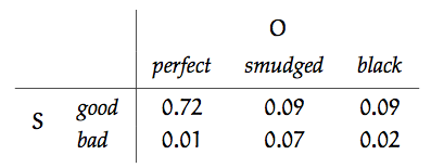
Now, conditioning on the actual observation, O_0 = \textit{perfect} , we extract the column corresponding to the observation, \{ 0.72, 0.01\} , and divide by the sum, 0.73 , to get the distribution

Here is a schematic version of this update rule, which is a good way to think about computing it by hand. Rather than creating the whole joint distribution and then conditioning by selecting out a single column, we just create the column we know we're going to need (based on the observation we got):

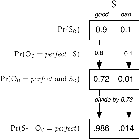
Because we will use it in later calculations, we will define B'_0 as an abbreviation:

that is, our belief that the system is in state s on the 0th step, after having taken the actual observation o_0 into account. This update strategy computes B'_0(s) for all s , which we'll need in order to do further calculations.

Now, we can think about the consequences of the passage of one step of time. We'd like to compute \Pr (S_1 \mid O_0 = \textit{perfect}) . Note that we are not yet thinking about the observation we'll get on step 1; just what we know about the machine on step 1 having observed a perfect copy at step 0.

What matters is the probability of making transitions between states at time 0 and states at time 1. We can make this relationship clear by constructing the joint probability distribution on S_0 and S_1 (it is actually conditioned on O_0 = \textit{perfect} ). So, \Pr (S_0, S_1 \mid O_0 = \textit{perfect}) can be constructed from \Pr (S_0 \mid O_0 = \textit{perfect}) (which, it is important to remember, is a distribution on S_0 ) and \Pr (S_1 \mid S_0) , which is our transition model:

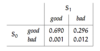
Now, we have never really known the value of S_0 for sure, and we can never really know it; we'd like to concentrate all of our information in a representation of our knowledge about S_1 . We can do that by computing the marginal distribution on S_1 from this joint. Summing up the columns, we get

This is an application of the law of total probability.

We'll give this distribution, \Pr (S_1 \mid O_0 = \textit{perfect}) , that is, everything we know about the machine after the first observation and transition, the abbreviation B_1 .

Here is a schematic version of the transition update:

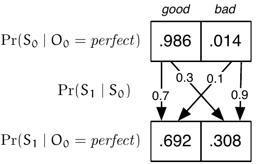
You can see that there are two ways the copier could be in a good state at time 1: because it was in a good state at time 0 (probability 0.986 ) and made a transition to a good state at time 1 (probability 0.7 ) or because it was in a bad state at time 0 (probability 0.014 ) and made a transition to a good state at time 1 (probability 0.1 ). So, the resulting probability of being in a good state is 0.986 \cdot 0.7 + 0.014 \cdot 0.1 = 0.692 . The reasoning for ending in a bad state is the same.

5.13) Our second copy

Now, let's imagine we print another page, and it's smudged. We want to compute \Pr (S_2 \mid O_0 = \textit{perfect}, O_1 = \textit{smudged}) . This can be computed in two stages as before. We start with B_1 , which already has the information that O_0 = \textit{perfect} incorporated into it. Our job will be to fold in the information that O_1 = \textit{smudged} , and then the passage of another step of time.

• Construct a joint distribution from B_1 and \Pr (O_1 \mid S_1) , and condition on O_1 = \textit{smudged} to get B'_1 . This is a Bayesian reasoning step.

• Construct a joint distribution from B'_1 and \Pr (S_2 \mid S_1) and marginalize out S_1 to get B_2 . This is a law-of-total-probability step.

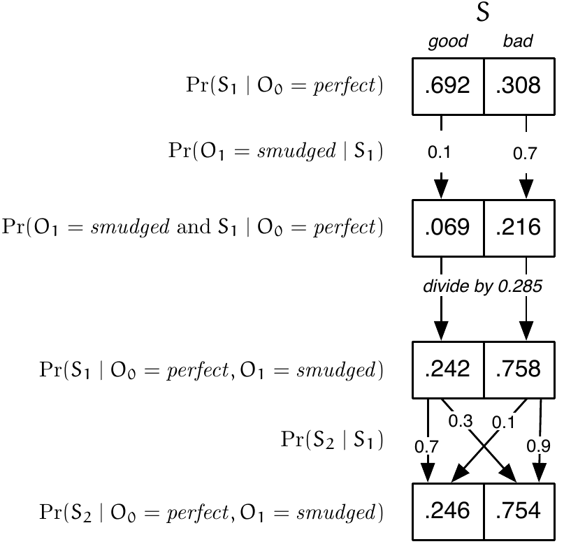
Ow. Now we're pretty sure our copy machine is no good. Planned obsolescence strikes again!

5.14) General state estimation

Now we'll write out the state-update procedure for HMMs in general. As a reminder, here are the random variables involved:

• State at each time S_0, \ldots , S_ T

• Observation at each time O_0, \ldots , O_ T

Here are the components of the model:

• Initial distribution \Pr (S_0)

• Observation distribution \Pr (O_ t \mid S_ t ) . Because the process is time-invariant, this is the same for all t .

• Transition distribution \Pr (S_{t+1} \mid S_ t) . Because the process is time-invariant, this is the same for all t . Think of i as selecting a particular conditional transition distribution to be used in the update.

Now, here is the update procedure. Assume that we have a belief state at time t , corresponding to \Pr (S_ t \mid O_{0..t-1} = o_{0..t-1}) . Then we proceed in two steps:

• Observation update, given o_ t :

  \Pr (S_ t \mid	O_{0..t} = o_{0..t})
  	= \frac{\Pr (O_ t = o_ t \mid S_ t) \Pr (S_ t \mid O_{0..t-1} =o_{0..t-1})}{\Pr (O_ t = o_ t\mid O_{0..t-1} = o_{0..t-1})}

• Transition update, given i_ t :

  \Pr (S_{t+1} \mid	O_{0..t} = o_{0..t})
  	= \sum _{r} \Pr (S_{t+1} \mid S_ t = r) \Pr (S_ t = r\mid O_{0..t} = o_{0..t})

A very important thing to see about these definitions is that they enable us to build what is known as a recursive state estimator. (Unfortunately, this is a different use of the term "recursive" than we're used to from programming languages). If we define our belief at time t ,

and our belief after making the observation update to be

then after each observation and transition, we can update our belief state, to get a new B_ t . Then, we can forget the particular observation we had, and just use the B_ t and o_ t to compute B_{t+1} . This is justified because the observations are conditionally independent given the state, and so this is like the example we saw earlier of using Bayes' rule to incorporate multiple pieces of evidence sequentially.

Algorithmically, we can run a loop of the form:

• Condition on actual observation O_ t = o_ t .

  B'(s) = \frac{\Pr (O_ t = o_ t \mid S_ t = s) B(s)}{\sum _ r\Pr (O_ t = o_ t \mid S_ t = r) B(r)}

• Make transition.

  B(s) = \sum _ r \Pr (S_{t+1} = s \mid S_ t = r) B'(r)

where B is initialized to be our initial belief about the state of the system.