6.01 Course Notes
2) Circuits
Table of Contents
- 2) Circuits
In conventional English, a circuit is a path or route that starts at one place and ultimately returns to that same place. The engineering sense of the word is similar. In electronics, a circuit is a closed path through which electrical currents can flow. The flow of electrical current through a flashlight illustrates the idea.

|

|
Three parts of the flashlight comprise the circuit: the battery, which supplies power, a bulb, which produces light when connected to the battery, and a switch, which can either be on (connected) or off (disconnected). The important feature of this circuit is that electrical currents flow through it in a loop, as illustrated in the right part of the figure above. When the switch is open, there is no path for current to flow; when the switch is closed, current begins to flow.
The rules that govern the flow of electrical current are similar to the rules that govern the flow of certain types of fluids; and it is often helpful to draw analogies between these flows. For example, the following figure illustrates the flow of blood through the human circulatory system.

The right side (from the person's viewpoint) of the heart pumps blood through the lungs and into the left side of the heart, where it is then pumped throughout the body. The heart and associated network of arteries, capillaries, and veins can be thought of and analyzed as a circuit. As with the flow of electrical current in the flashlight example, blood flows through the circulatory system in loops: it starts at one place and ultimately returns to that same place.
As we learn about circuits, we will occasionally point out analogies to fluid dynamics for two reasons. First, we all have developed some intuition for the flow of fluid as a result of our interactions with fluids as a part of everyday experience. We can leverage the similarity between fluid flow and the flow of electrical current to increase our intuition for electrical circuits. Second, the analogy between electrical circuits and fluid dynamics is a simple example of the use of circuits to make models of other phenomena. Such models are widely used in acoustics, hydrodynamics, cellular biophysics, systems biology, neurophysiology, and many other fields.
Electrical circuits are made up of components, such as resistors, capacitors, inductors, and transistors, connected together by wires. You can make arbitrarily amazing, complicated devices by hooking these things up in different ways, but in order to help with analysis and design of circuits, we need a systematic way of understanding how they work.
As usual, we can't comprehend the whole thing at once: it's too hard to analyze the system at the level of individual components, so, again, we're going to build a model in terms of primitives, means of combination, and means of abstraction. The primitives will be the basic components, such as resistors and op-amps; the means of combination is wiring the primitives together into circuits.
We'll find that abstraction in circuits is different than in software or LTI systems. You can't think of a circuit as "computing" the voltages on its wires: if you connect it to another circuit, then the voltages are very likely to be different. However, you can think of a circuit as enforcing a constraint on the voltages and currents that enter and exit it; this constraint will remain true, no matter what else you connect to the circuit.
2.1) Electrical Circuits
Our electrical abstraction is based on two major types of pieces: nodes and components. In general, a circuit consists of several components connected by nodes.
Voltage is a difference in electrical potential between two different nodes in a circuit. We will often pick some point in a circuit to use as a reference; we will call this reference the ground node, and say that it is at 0 electrical potential. Since voltage is a relative concept, we could pick any point in the circuit and call it ground, and all the relative voltages would remain the same. The unit of potential difference, or voltage, is the Volt (not too surprisingly), which is abbreviated as V.
Current is a flow of electrical charge through a path in the circuit. Positive charge carriers (e.g., ions of inert gases like Neon) flowing in a certain direction correspond to positive current flowing in that direction. In metals, the charge carriers happen to have negative charge, so the direction of current flow in this case is opposite to that of the flow of charge carriers. The unit of current is the Ampere (often just called amp for short), which is abbreviated as A.
What physical mechanisms cause flow? Blood circulates due to pressures generated in the heart. Hydraulic pressure also moves water through the pipes of your house. In similar fashion, voltages propel electrical currents. A voltage can be associated with every node in a circuit, and it is the difference in voltage between two nodes that drives electrical current between the nodes; absolute voltage is not important (or even well defined).
2.1.1) Nodes
A node is any electrically connected region in space (such as a wire, a piece of metal, or several connected wires). All points within a node are at the same electrical potential.
For practical purposes, we can think about a node as a set of points in a circuit that are all connected by only a wire1. For example, the following circuit has three components (represented by the boxes below), which are connected by two nodes; one node is colored in red, and the other is colored in blue.

2.1.2) Components
A component describes relationships between nodes, as well as the way that current flows between nodes. In a general sense, a component is anything that connects to multiple nodes2.
An arbitrary component is generally drawn as a box, as in the example circuit above. We will see examples of specific components in the following section, but for now, we will talk more generally.
We will start by considering a simple set of components that have two terminal points (two connection points into the circuit). We will refer to such components as one-ports. Each component has a current flowing through it, as well as a voltage difference across its terminals. Each type of component has some special characteristics that govern the relationship between its voltage and current. In 6.01, we will restrict our attention to components that exert a linear constraint between their current and voltage.
Consider the following one-port component:

The variable v_1 represents the potential difference between the two nodes on either side of the component. In particular, because the "plus" sign (+) is on the top node, v_1 represents the potential difference between the top node and the bottom node. It is important to note that the definition of the voltage variable v_1 specifies a reference direction. The voltage can be either positive or negative in value. If the top node is at a potential 8 Volts higher than the bottom node, then v_1 = 8V; if, however, the top node is at a potential 8 Volts lower than the bottom node, then v_1 = -8V.
The variable i_1 represents the current flowing through the component, in the direction indicated by the arrow. As with v_1, i_1 provides a reference direction, and does not constrain the actual direction in which current flows in the circuit. In this example, if current is actually flowing downward at 2 Amps, then i_1 = 2A; if, however, current is actually flowing upward at 2 Amps, then i_1=-2A. Importantly, the current flowing from the top node into the component is identical to the current flowing out of the component into the bottom node (i.e., i_1 is found on both sides of the component in the same direction).
It bears repeating that the voltage and current variables for each component (for example, v_1 and i_1 for this component) are frames of reference that we draw, and do not necessarily imply the actual direction in which current is flowing, or the actual direction of the potential drop. As long as you are consistent when dealing with these variables, you should arrive at the same result at the end of your analysis, regardless of your reference frame.
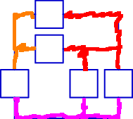
How many components and how many nodes does the following circuit have?

Show/Hide
This circuit contains 5 components (represented by the boxes), and 3 nodes (the regions between components that are connected only by wires). The nodes are highlighted in three different colors below: red in the upper-right, orange in the upper-left, and magenta on the bottom:
2.2) Component Types
In general, each electrical component imposes a relation between the voltage difference of its two nodes, and on the current flowing through it. This relation is called a constitutive relation (or constitutive equation). For now, we will introduce two types of components, each with a distinct constitutive equation3.
2.2.1) Voltage Source
A voltage source is a component whose voltage is a constant (i.e., \Delta v = V_0) independent of the current flowing through it. We will denote a voltage source by a circle enclosing plus and minus signs to denote voltage. A number beside the voltage source will indicate the constant voltage generated by the source, as indicated below:

This voltage source will make sure that the potential difference between its top node and its bottom node is always V_0. Importantly, the current flowing through the voltage source is unconstrained by the source itself; rather, it is constrained by the other components to which this source is connected. The current flowing through the voltage source will be whatever it needs to be, in order to maintain this constraint on its voltage (it can be positive, negative, or zero!).
Below, we plot this device's I-V Characteristic; this is a graph that shows the relation between the variables v and i. Note that, for this particular component, the current can take any value; the voltage will always be V_0. The plot below shows the relation for a 1.5 Volt voltage source (V_0 = 1.5V).

2.2.1.1) What's In A Name?
We call this idealized device a voltage source, but it is important to keep in mind that it does not always act as a power source to the circuit. In many ways, it would make more sense to call this device a voltage constraint; regardless of whether or not it is supplying power to the circuit, it always constrains the voltage across it to be constant.
Sometimes, as we will see in lab, it makes sense to model certain things as voltage sources (i.e., as exerting a constraint on a voltage), even if they are not providing power to the circuit.
2.2.2) Resistor
In a resistor, the voltage is proportional to the current. The constant of proportionality the relates the two is the resistance4 R. This relation, \Delta v = iR, is called Ohm's Law. Importantly, voltage always drops in the direction of current flow in a resistor. So the relationship really is that v_+ - v_- = iR, and the sign matters!
The resistance R has units of Ohms = Volts per Ampere. Ohms are abbreviated as \Omega. We will denote a resistor as follows; a number to the side of the resistor indicates its resistance.

Below, we plot the I-V Characteristic for a resistor whose resistance is R = 0.5\Omega.

How does the slope of this curve relate to the resistance R of the resistor?
Show/Hide
Since we are looking at I with respect to V, the slope of this line is 1/R.
2.2.3) Ideality
It is worth noting that these components are idealized models, and are not exactly the way things work in the real world. For example, there is no such thing in the real world as an ideal voltage source (whose voltage is always constant); that said, batteries often behave close enough to this ideal that we can model them as ideal voltage sources5.
Similarly, ideal wires and ideal resistors do not actually exist, but the components we will use in lab are close enough to the idealized models that modeling them this way makes good sense (our problems would certainly grow much more complicated if we modeled these components more accurately, and, for our purposes, the results would be similar, so this would not be worth the effort!).
2.3) Multiple Components
When multiple components exist in the same circuit, each exerts its own constraints on the currents and node voltages in the circuit. For simple circuits, it is relatively simple to see how these constraints interact. For example, let's consider solving for the current i flowing through the resistor in the following circuit:

The voltage source on the left will ensure that there is a 2 Volt difference between the top node and the bottom node. Since the resistor shares those same two nodes, we know that there must also be a 2 Volt drop across the resistor (the resistor's top terminal is at a potential 2 Volts higher than its bottom terminal). Since, by Ohm's Law, the current flowing through the resistor will be equal to the voltage drop across the resistor divided by its resistance, we know that this current must be i = 2V/2\Omega = 1A.
We can also think about this graphically. We know that the nodes on either side of the resistor must satisfy the constraints of both the voltage source and the resistor. Plotting both components' I-V Characteristics on the axes below, we see that there is exactly one point in I-V space at which both constraints can be satisfied (this point is highlighted in red), which corresponds to our solution from above.

2.3.1) Conservation Laws
For simple circuits, thinking about how the individual components' constraints interact is relatively easy. When you start to construct circuits from multiple components, however, additional laws must be applied in order to relate how the arrangement of the components affects the various voltages and currents in the circuit.
2.3.1.1) Kirchoff's Current Law
Kirchoff's Current Law ("KCL" for short) can be thought of as the electrical form of conservation of mass. Electrical charge cannot be created nor destroyed in an electrical circuit. This applies to both components and nodes. We already saw evidence of this when we said that the current into a component is the same as the current out of that component on the other side in the previous section. Similarly, if a certain amount of current is flowing into a node, an identical amount must also be flowing out through some other channel in order to maintain equilibrium at that node.
Consider the case where we have three components connected as in the following diagram:

The first thing we should notice is that all three components are connected to the same two nodes. Now let's consider the currents flowing through each of these components:

KCL states that the sum of all currents flowing out of a node must be zero. For the top node, we can say that i_1+i_2+i_3=0. For the bottom node, we can say that -i_1-i_2-i_3=0. The positive/negative difference comes from the fact that in the top node, all currents are defined as flowing out of that node, while in the bottom case they are all flowing into the node. Note that mathematically these two statements are equivalent.
If i_1 were defined as having the opposite direction (so that it is defined as flowing up instead of down), what would our KCL equation be then in terms of the currents?
Show/Hide
-i_1+i_2+i_3=0
A circuit is divided into the part that is inside the dashed red box (below) and the part that is outside the box (not shown). Find an equation that relates the currents i_1 and i_2 that flow through the dashed red box.

Show/Hide
i_1 = -i_2
A more complicated circuit is shown inside the red box below. Find an equation that relates the currents i_1, i_2, and i_3 that flow through the dashed red box.

Show/Hide
-i_1 = i_2 + i_3
2.3.1.2) Kirchoff's Voltage Law
Kirchoff's Voltage law ("KVL" for short) states that for any complete loop in a circuit, the total component voltage encountered when traversing that loop must be zero. That is, starting at any point in a circuit and following a closed path back to that point, accounting for the voltage drop across each component encountered along the way, you must end up back at the same potential.
The following set of voltages are not consistent with Kirchhoff's voltage laws but can be made consistent by changing just one. Which one should you change, and what should its new value be??

Show/Hide
The bottom-center component's voltage drop should be 1V instead of 2V.
2.4) Equivalent Circuits
In an earlier section, we introduced the idea of a one-port (a component with two terminals):

Current enters one terminal (+) and leaves the other (-). The one-port constrains the relationship between the current i_1 and the voltage v_1. We have already seen several examples of one-ports, and we have seen how these components constrain the current flowing through them, as well as the voltage drop across them.
In this section, we will find that we can often simplify circuits by replacing certain combinations of components in the circuits with equivalent one-ports. Often, such methods can be applied again on the resulting circuit to produce something even simpler.
2.5) Series and Parallel Combinations
Two "special cases" of equivalent circuits are series and parallel combinations of components.
2.5.1) Series Combination
The first type of combination we will explore involves two components connected in series. Components are considered to be connected in series if they share one node that is not shared with any other component that draws or injects current from/to that node. By Kirchoff's current law, the current flowing through one such component must be the same as the current flowing through the other.
For example, the following two components are connected in series because they share a central node, and no other components are connected there:

We can think about this circuit itself as exerting a constraint on two new variables, which are labeled I and V in the diagram below:

In this circuit, we have:
- I = i_1 = i_2, and
- V = v_1 + v_2
So we can think of this combination as exerting a single linear constraint on V and I, rather than exerting two constraints (one on v_1 and i_1, and another on v_2 and i_2).
Consider the following circuit, which consists of a voltage source connected in series with a resistor.

Which of the following I-V characteristics describes the relationship between V and I?

|

|

|

|

|

|
Show/Hide
The voltage across the voltage source is always going to be 1V (regardless of current), and the voltage drop across the resistor is going to be v_r = I\cdot1\Omega. The total voltage drop V, then, must be V = I\cdot1\Omega + 1V.
When I=0, V must be 1V; as I changes, V also changes (according to the equation above). Only one graph has these properties:

We could also have solved directly for I in terms of V and gotten the following, which also leads us to that graph:
2.5.1.1) Series Combination of Resistors
A useful special case of the rules above for series combination involves two resistors connected in series. Two resistors in series can be replaced with a single resistor R_s to yield an equivalent circuit:

|

|
If i and v are constrained in the same way in the two circuits above, what is the relationship between R_1, R_2, and R_s?
Show/Hide
By Ohm's Law, we know that v = iR_s. We also know that v is the sum of the voltage drops across R_1 and R_2, so we also have: v = iR_1 + iR_2.
Since these are both expressions for v, we can say that:
When analyzing circuits, it may be useful to look for resistors connected in series. You can replace these two resistors with a single equivalent resistor (whose resistance we just found above), which may simplify your analysis.
Resistors in series also act as voltage dividers. That is, they split voltages in predictable ways. Consider the following circuit:

In this circuit, we have:
Notice that the voltage drop across R_2 goes like the fraction of the total resistance that comes from R_2.
Note that this relation only holds if the two resistors are connected in series (if the current flowing through each of the resistors is exactly the same).
Consider the series combination of a 500\Omega resistor and a 5\Omega resistor. Which of the following is closest to the equivalent resistance of this combination?

- 5\Omega
- 250\Omega
- 500\Omega
- 1k\Omega
Show/Hide
In this combination, we know that the current running through the two resistors must be the same (since they are connected in series), so we are interested in the extent to which each resistor contributes to the voltage drop across the combination.
Since \Delta v = iR, the 5\Omega resistor accounts for less than 1% of the voltage drop across the combination. Thus, it can be largely ignored.
The exact equivalent resistance, as we found in the previous section, is 505\Omega, but we can approximate the combination as just the 500\Omega resistor since the smaller resistor contributes so little.
In the last "check yourself" question, we noticed that we can sometimes approximate the series combination of two resistors with resistances R_1 and R_2 as \text{max}(R_1, R_2). When does this approximation break down?
Show/Hide
This approximation holds best when R_1 and R_2 are very different in magnitude. As R_1 gets closer to R_2, this approximation breaks down.
And when R_1 = R_2, it isn't very good at all, since the series combination of R_1 and R_2 is, in that case, 2R_1.
2.5.2) Parallel Combination
The second type of combination we will explore involves two components connected in parallel. Components are considered to be connected in parallel if there exists a closed loop containing only those two components. By Kirchoff's Voltage Law, the voltage drop across these two components must be the same. Another way to think about this is that components are considered to be connected in parallel if they share both endpoint nodes.
For example, the following two components are connected in parallel:

We can think about this circuit itself as exerting a constraint on two new variables, which are labeled I and V in the diagram below:

In this circuit, we have:
- I = i_1 + i_2
- V = v_1 = v_2
As before, we can think about this combination as exerting a single linear constraint on V and I, rather than exerting two constraints.
Consider the following circuit, which consists of a voltage source connected in parallel with a resistor.

Which of the following I-V characteristics describes the relationship between V and I?

|

|

|

|

|

|
Show/Hide
The voltage across the voltage source is always going to be 1V (regardless of current), which is the same contraint that the voltage source alone would exert!
Note that, in order for this to be true, the current through the resistor must always be 1A flowing downward, regardless of the value of I. This will be remedied by the voltage source, which will source (or sink!) as much current as it must in order to maintain the 1A current flowing through the resistor.
For example, if I=0, the voltage source will have 1A of current flowing upward through it, and all of that current will flow back down through the resistor. If I=0.5A, the coltage course will provide an additional 0.5A of current. If I=2A, something interesting happens; the voltage source will not provide current, but, rather will act as a current sink; in this case, it will have 1A of current flowing downward through it.
What is an example of two components that cannot be connected in parallel without violating the conservation laws above?
Show/Hide
Connecting two voltage sources in parallel, each of which has a different voltage, would lead to a violation of Kirchoff's voltage law.
2.5.2.1) Parallel Combination of Resistors
A useful special case of the rules for parallel combination involves two resistors connected in parallel. Two resistors in parallel can be replaced with a single resistor R_p to yield an equivalent circuit:

|

|
If i and v are constrained in the same way in the two circuits above, what is the relationship between R_1, R_2, and R_p?
Show/Hide
We know that the current i is the sum of the currents running through R_1 and R_2, which are (by Ohm's Law) v / R_1 and v / R_2, respectively. We also know that this current is the same as the current running through R_p, so we have:
Pulling out a common factor, we have:
How does R_p compare in magnitude to R_1 and R_2?
Show/Hide
R_p must be less than or equal to R_1, and it must also be less than or equal to R_2.
When analyzing circuits, it may be useful to look for resistors connected in parallel. You can replace these two resistors with a single equivalent resistor (whose resistance we just found above), which may simplify your analysis.
Resistors in parallel also act as current dividers. That is, they split currents in predictable ways. Consider the following circuit:

In this circuit, we have:
Notice that the current flowing through one resistor goes like the fraction of the resistance contributed by the other resistor.
Note that this relation only holds if the two resistors are connected in parallel (if they share both endpoint nodes).
Consider the parallel combination of a 500\Omega resistor and a 5\Omega resistor. Which of the following is closest to the equivalent resistance of this combination?

- 5\Omega
- 250\Omega
- 500\Omega
- 1k\Omega
Show/Hide
In this combination, we know that the voltage across the two resistors must be the same (since they are connected in parallel), so we are interested in the extent to which current flows through each resistor.
Since i = \Delta v / R, the 500\Omega resistor accounts for less than 1% of the current flow through the combination. Thus, it can be largely ignored.
The exact equivalent resistance is tedious to solve, but we can approximate the combination as just the 5\Omega resistor since so little current flows through the bigger resistor.
In the last "check yourself" question, we noticed that we can sometimes approximate the parallel combination of two resistors with resistances R_1 and R_2 as \text{min}(R_1, R_2). When does this approximation break down?
Show/Hide
This approximation holds best when R_1 and R_2 are very different in magnitude. As R_1 gets closer to R_2, this approximation breaks down.
And when R_1 = R_2, it isn't very good at all, since the parallel combination of R_1 and R_2 is, in that case, R_1 / 2.
In the following graph, one line represents the equivalent resistance of the parallel combination of a resistor R and a 10\Omega resistor vs R, and the other represents the equivalent resistance of a series combination of R and a 10\Omega resistor vs R. Which line is which? How can you tell?

Show/Hide
The green line here represents the series combination (notice that, for small values of R, the combination is around 10\Omega, and for large values of R, the combination is around R).
The blue line represents the parallel combination (notice that, for small values of R, the combination is around R, and for large values of R, the combination is around 10\Omega).
2.6) Solving Circuits
Combining the ideas from the previous sections, we can develop a process for solving arbitrary circuits, which we will explain here and demonstrate in 3 sample circuits. Our process is:
-
Make a note of all the nodes in the circuit, and pick one to be our reference node. All other node potentials will be measured with respect to this node. As a result, the potential at the reference node is 0V (with respect to itself).
-
Look for a constitutive equation with exactly one unknown value. If such an equation exists, solve for the unknown value, add it to the diagram as a known, and jump to step 6.
-
Look for a KCL equation with exactly one unknown current. If such an equation exists, solve for the unknown current, add it to the diagram as a known, and jump to step 6.
-
If you made it through steps 2 and 3 without finding an equation with exactly one unknown, look for patterns that can simplify the circuit (series/parallel combinations, etc, which are discussed in the following sections), and continue from step 2.
-
Last Resort: If you made it though steps 2, 3, and 4 without finding any simplifications that can be made, then write a system of constitutive and KCL equations in terms of node potentials, and solve6.
-
If the circuit is completely solved, congratulations! If not, continue from step 2.
Step 2 asks to find components whose constitutive equations have exactly one unknown. How can we apply this to the two component types we have talked about so far, voltage sources and resistors?
Show/Hide
If we have a voltage source with a known voltage and we know the potential at one of its terminal nodes, we can solve for the potential at its other terminal node.
If we have a resistor with a known resistance and we know the potential at one terminal node, as well as the current, we can solve for the potential at its other terminal node.
If we have a resistor with a known resistance and we know the potentials at _both_ terminal nodes, we can solve for the current through the resistor.
2.6.1) Example Circuit 1
Let's take a look at how applying the algorithm described above applies to solving a real circuit. Consider solving for all voltages and currents in the following example circuit:

- We can start with step 1, labeling one of the nodes in the circuit as our reference point. Here, we will pick the bottom node (this will be convenient because it will make calculating a lot of the other potentials easier, particularly those at the "top" of the voltage sources). We can label this node as being at 0V potential. Note that the entire bottom wire is now at 0V potential, even though the label is only at one particular spot.

- Now we are in step 2, and we look for components whose constitutive equations have only one unknown. One of these is the 5\Omega resistor. We know, by Ohm's Law, that \Delta v = iR. Here, we know that R = 5\Omega, and we know that i = 3A. Solving, we know that \Delta v = 15V. Since the bottom of the resistor is at 0V potential, then the top of the resistor must be at 15V potential (15V higher than its bottom node):

- Back in step 2, we again look for components whose constitutive equations have only one unknown. The vertical 2\Omega resistor can be solved in much the same way we solved the 5\Omega resistor. If the current through the resistor is 3A and its resistance is 2\Omega, then the voltage drop across it must be 6V. And because the bottom node is at 0V potential, we know that the top node must be at 6V potential:

- Back in step 2, we again look for components whose constitutive equations have only one unknown. With the new information we got from solving the first two resistors, we can now solve the horizontal 1\Omega resistor. Here we know that the voltage drop across the resistor is 9V (left-to-right), and the resistance is 1\Omega. Therefore, the current flowing (left-to-right) through the resistor must be \Delta v / R = 9V/1\Omega = 9A.

- Back in step 2, we again look for components whose constitutive equations have only one unknown. However, no such components exist, and so we move on to looking for a KCL equation with only one unknown current. In fact, there are a couple of them! Let's start with the node at the top of the 5\Omega resistor. Here, we have 9A leaving to the right and 3A leaving to the bottom. By KCL, the total current entering the node must equal the total current exiting the node, and so we know that there must be 12A entering the node from the left.

- We can apply a similar analysis to the node at the top of the 2\Omega resistor. Here, we have 9A entering from the left and 3A leaving to the bottom. By KCL, the total current entering the node must equal the total current exiting the node, and so we know that there must be 6A leaving the node to the right.

- By KCL at the top-left and top-right corners, we also now know that I_1 = -12A, and that I_2 = 6A. We can verify by checking KCL at the bottom node (and, good for us, it checks out, since the currents sum to 0!).

- Now we know every current in the circuit (hooray!), so we have exhausted the usefulness of KCL in this circuit. But there are still some potentials and component values to solve, so we can look, once again, for components whose equations have only one unknown. In this case, we can start with the 4\Omega resistor in the upper-left. We know, by Ohm's Law, that the voltage drop must be 4\Omega \cdot 12A = 48V (that is, the left-hand node's potential must be 48V higher than the right-hand node's potential). Since the right-hand node is at 15V, the left-hand node must be at 15V + 48V = 63V.

- We can apply a similar analysis to the horizontal 2\Omega resistor in the upper-right. We know, by Ohm's Law, that the voltage drop must be 2\Omega \cdot 6A = 12V (that is, the left-hand node's potential must be 12V higher than the right-hand node's potential). Since the left-hand node is at 6V potential, we know that the right-hand side must be at 6V - 12V = -6V. This might seem strange, but all it means is that the node in the upper-right corner is at a potential that is 6V lower than our reference node. Had we chosen a different reference, we could have ended with all positive potentials.

- Now we are almost done! We are back to looking for constitutive equations with exatcly one unknown, and both of the remaining voltage sources fall in thar category. For the left-most voltage source, for example, we know that the difference between the top and bottom nodes' potentials must be 63V, and it must also be V_1. Therefore, V_1 = 63V.

- And for the right-most voltage source, we know that the difference between the top and bottom nodes' potentials must be -6V, and it must also be V_2. Therefore, V_2 = -6V.

And we're done! This might look like a lot of steps when written out this way, but each of those steps was a relatively simple operation (usually, it amounted to a single division, multiplication, or addition!). So by taking this sequence of small steps, we were able to solve the entire circuit!
2.6.2) Example Circuit 2
Consider solving for all currents and voltages in the following circuit:

- As before, we can start by labeling one node as our reference (0V). Again, we will choose the bottom node:

- Since the bottom node of the voltage source is at 0V potential, we know that the top node of the voltage source must be at 10V:

- Now at this point, we encounter a problem: all of the KCL equations and constitutive equations have more than one unknown. So now we enter step "4" of the process described above: looking for ways to simplify the circuit using equivalent circuits. Notice first that the bottom two resistors are connected in parallel (they share both terminal nodes). Thus, we can replace them with an equivalent resistance:

- Even after that simplification, we don't have any trivially-solveable equations, and so we go back to step 4. After our simplification from a moment ago, we now have two resistors connected in series. So we can replace that combination, too, with an equivalent resistance:

- After those simplifications, we now have a resistor whose constitutive equation has exactly one unknown (the current!). We can, therefore, solve for the current through this resistor. We know the potential difference is 10V and the resistance is 1.5k\Omega, so the current is 10/1500 = 2/300 \text{A} = 20/3 \text{mA}.

- Now that we have solved for the current, we can "undo" one step of our abstraction, breaking the series combination back apart:

- Now, the top resistor's equation has exactly one unknown: the potential in between the two resistors. We know that the resistance is 1k\Omega, and that the current is 2/300 A. So the voltage drop must be 1k\Omega \cdot 2/300A = 20/3 V. But since the top node is at 10V potential, this value is not simply the potential at the center node. Rather, that potential is 10V - 20/3V = 10/3V.

- Now, again, we seem to be out of equations with only one unknown. But if we break apart our first parallel combination back into its original components, we will see some more avenues open up:

- Now we have two resistors, and for each, we know the voltage drop and the resistance. So we can solve for the current through each. For each, the current is 10/3V / 1k\Omega = 1/300 A. We can verify by checking KCL at the center node (hooray! it does indeed check out).

This circuit was a little more complicated to think about than our first example, because it required finding several equivalent circuits along the way. But our method still brought us to the right solution!
With time and practice, noticing these kinds of combinations will become faster and easier!
2.6.3) Example Circuit 3
Consider solving for all currents and voltages in the following circuit:

- As always, we can start by picking a node as a reference. The bottom node looks like a good choice, since that will allow us to solve for the potentials at two other nodes easily.

- We then have two components whose equations have exactly one unknown: each of the voltage sources. We can, therefore, solve for the potential at the top of each:

- Now we look for other components whose equations have exactly one unknown, and we find none. We look for series/parallel combinations or other simplifications, and find none. So now we hit the last resort condition in our algorithm: we must write an equation. In particular, an easy equation to write is a KCL equation at a node whose potential we don't know (this is particularly useful if we can write it in terms of node potentials using Ohm's Law). In this case, there is exactly one. Let's label our unknown potential as x:

- We can also think about the currents flowing into/out of this node. We don't exactly know which direction they are flowing yet (that depends on x!), but we can pick a reference direction for each current. We may find out later that these directions are wrong, but that's okay! So here we will pick directions for the currents:

- We could give names to these currents (call them i_1, i_2, and i_3, maybe), but we can also write expressions for them in terms of node potentials using Ohm's Law:

- By KCL, we know how these currents must be related, and we can solve for the potential x:

- Once we know x, we can solve for the actual currents in the circuit. We can either just substitute x=3V into the expressions we found earlier for the currents, or we can go back and notice that, knowing that center potential, we have 3 resistors whose equations now each have exactly one unknown. Also note that one of our directions was initially wrong (the current through he 2\Omega resistor is actually flowing right-to-left!), but that's okay.

2.7) Summary (The Story So Far)
So far in this chapter, we introduced the idea of circuits, with a particular focus on electrical circuits. We introduced the concepts of nodes and components, and we saw two different examples of specific common components: voltage sources and resistors. We noticed that when multiple components are connected together, all of their constraints must still be satisfied.
We also introduced the one port abstraction, whereby components are represented by their I-V Characteristic curve. We saw how multiple components could be replaced with equivalent one-ports, in particular by looking at series and parallel combinations.
Finally, we introduced a general process for solving circuits and looked at a couple of specific examples of using that method to solve somewhat-complicated circuits.
Footnotes
1Wire is typically made from metals through which electrons can flow to produce electrical currents. Generally, the strong forces of repulsion between electrons prevent them from accumulating in wires. However, thinking about nodes as wires is only an approximation, since actual physical wires can have more complicated electrical properties.
2Such as a resistor, a motor, a battery, or a squirrel foolishly bridging two power lines.
3In later sections, we will introduce additional types of components.
4As the name suggests, this is a measure of how strongly the component resists the flow of current
5There may be times, though, when modeling a battery as a voltage source is not enough, and we have to use a more complicated model of a battery.
6This is almost always a more difficult way to solve the circuit, and should be a rarity in 6.01!